This homework aims at giving you some experience with Python’s array computing and plotting features.
1. The while-loop implementation of a for-loop. Consider the following mathematical function resembling a Hat function,
\[f(x) = \begin{cases} 0 ~, & \text{if}~~ x<0 \\ x ~, & \text{if}~~ 0\leq x <1 \\ 2-x ~, & \text{if}~~ 1\leq x <2 \\ 0 ~, & \text{if}~~ x \geq 2 \\ \end{cases}\]A scalar implementation of this function would be,
def hatFunc(x):
    if x < 0:
        return 0.0
    elif 0 <= x < 1:
        return x
    elif 1 <= x < 2:
        return 2 - x
    elif x >= 2:
        return 0.0
Write a vectorized version of this function. (Hint: you may need numpy’s logical_and method for building the vectorized version of this function.)
2. The vertical position $y(t)$ of a ball thrown upward is given by $y(t)=v_0t-\frac{1}{2}gt^2$, where $g$ is the acceleration of gravity and $v_0$ is the initial vertical velocity at $t=0$. Two important physical quantities in this context are the potential energy, obtained by doing work against gravity, and the kinetic energy, arising from motion. The potential energy is defined as $P=mgy$, where $m$ is the mass of the ball. The kinetic energy is defined as $K=\frac{1}{2}mv^2$, where $v$ is the velocity of the ball, related to $y$ by $v(t)=y’(t)$.
Write a program that can plot $P(t)$ and $K(t)$ in the same plot, along with their sum $E = P + K$. Let $t\in[0,2v_0/g]$. Write your program such that $m$ and $v_0$ are read from the command line. Run the program with various choices of $m$ and $v_0$ and observe that $P+K$ always remains constant in this motion, regardless of initial conditions. This is in fact, the fundamental principle of conservation of energy in Physics.
3. Integration by midpoint rule: The idea of the Midpoint rule for integration is to divide the area under a curve $f(x)$ into $n$ equal-sized rectangles. The height of the rectangle is determined by the value of $f$ at the midpoint of the rectangle. The figure below illustrates the idea,
To implement the midpointrule, one has to compute the area of each rectangle, sum them up, just as in the formula for the Midpoint rule,
\[\int^b_a f(x) dx \approx h\sum^{n-1}_{i=0} f(a+ih+0.5h) ~,\]where $h=(b-a)/n$ is the width of each rectangle. Implement this formula as a Python function midpoint(f, a, b, n) and test the integrator with the following example input mathematical functions.
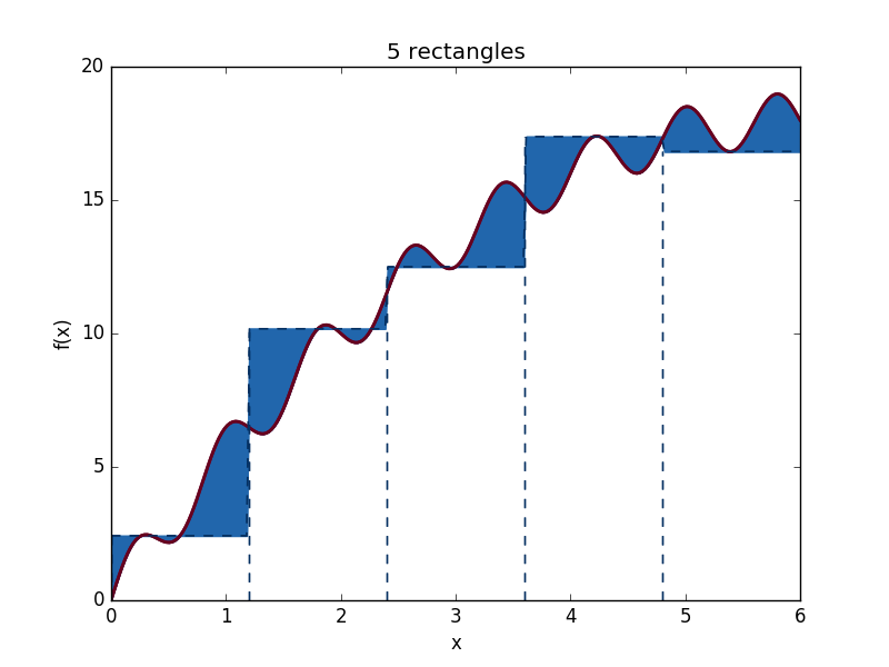
\[\begin{align*} f_1(x) &= exp(x) ~,~ \text{for integration range } ~ [0, \log(3)] \\\\ f_2(x) &= cos(x) ~,~ \text{for integration range } ~ [0, \pi] \\\\ f_3(x) &= sin(x) ~,~ \text{for integration range } ~ [0, \pi] \\\\ f_4(x) &= sin(x) ~,~ \text{for integration range } ~ [0, \pi / 2] \\\\ \end{align*}\]4. Visualize approximations in the Midpoint integration rule Now consider the following function,
\[f(x) = x(12-x)+\sin(\pi x) ~~,~~ x\in[0,10] ~,\]which we wish to integrate using the midpoint integrator that you wrote in the previous example. Now write a new code that visualizes the midpoint rule, similar to in the following figure. (Hint: you will need to use the Matplotlib function fill_between and use this function to create the filled areas between f(x) and the approximating rectangles)