This homework aims at giving you some experience with Python’s tools for interacting with the World Wide Web and writing Monte Carlo simulations.
Update: As I discussed in class, in order to avoid creating potential traffic on Professor Butler’s webpage, I have now uploaded all the necessary files on this address (don’t click on the links in this table, because it will take you to Professor Butler’s repository for this data. I have all the data already saved in our domain locally). So now, your goal is to first read the event-ID HTML table from
https://www.cdslab.org/ECL2017S/homework/9/swift/bat_time_table.html.
Then, use the event-IDs in this table to generate web addresses like:
https://www.cdslab.org/ECL2017S/homework/9/swift/GRB00100433_ep_flu.txt
in order to download these .txt files from the web. The rest of the homework is just as you would have done this problem as descibed below.
1. Reading scientific data from web. Consider the webpage of Professor Nat Butler at Arizona State University. He has successfully written Python piplines for automated analysis of data from NASA’s Swift satellite. For each Gamma-Ray Burst (GRB) detection that Swift makes, his pipline analyzes and reduces data for the burst and summarizes the results on his personal webpage, for example in this table.
(A) Write a Python function named fetchHtmlTable(link,outputPath) that takes two arguments:
- a web address (which will be this: http://butler.lab.asu.edu/swift/bat_time_table.html), and,
- an output path to where you want the code save the resulting files.
One file is exact HTML contained in the input webpage address, and a second file, which is the Table contained in this HTML address. To parse the HTML table in this address, you will need the Python code parseTable.py also available and explained on this page. This parsed HTML table, will be in the form of a list, whose elements correspond to each row in the HTML table, and each row of element of this parsed table is itself another list, that contains the columns of the HTML table in that row. Output this table as well, in a separate file, in a formatted style, meaning that each element of table in a row has a space of 30 characters for itself (or something appropriate as you wish, e.g., '{:>30}'.format(item)). You can see an example output of the code here for the HTML output file, and here for parse HTML table.
(B) Now, if you look at the content of the file that your function has generated (once you run it), you will see something like the following,
                   GRB (Trig#)               Trig_Time (SOD)               Time Region [s]                          T_90                          T_50                       rT_0.90                       rT_0.50                       rT_0.45                          T_av                         T_max                        T_rise                        T_fall                           Cts                       Rate_pk                          Band
       GRB170406x   (00745966)                     44943.130                -40.63->887.37              881.000 +/-7.697             549.000 +/-25.558             280.000 +/-13.432              124.000 +/-5.751              109.000 +/-4.997             433.667 +/-15.557            877.870 +/-367.494            890.500 +/-366.900              0.000 +/-366.630                6.082 +/-0.344               0.018 +/-0.0065                     15-350keV
       GRB170402x   (00745090)                     38023.150                  54.35->66.35                9.000 +/-2.096                5.000 +/-1.490                7.000 +/-1.535                4.000 +/-0.640                3.000 +/-0.559               60.964 +/-1.316               58.850 +/-2.417                1.500 +/-2.894                7.500 +/-2.720                0.162 +/-0.045               0.022 +/-0.0106                     15-350keV
       GRB170401x   (00745022)                     68455.150                 -19.63->71.49               78.880 +/-5.224               39.440 +/-4.168               41.480 +/-3.823               18.360 +/-1.585               16.320 +/-1.341               29.541 +/-2.857              24.910 +/-24.386              37.740 +/-24.251              41.140 +/-23.977                1.181 +/-0.122               0.024 +/-0.0130                     15-350keV
       GRB170331x   (00744791)                      6048.440                 9.835->35.875               20.160 +/-1.285               10.290 +/-0.914               14.070 +/-1.041                5.880 +/-0.415                5.040 +/-0.359               21.461 +/-0.598               12.460 +/-5.633                0.525 +/-5.718               19.635 +/-5.840                1.875 +/-0.154               0.134 +/-0.0408                     15-350keV
Now write another function that reads the events’ unique numbers that appear in this table in parentheses (e.g., 00745966 is the first in table), and puts this number in place of event_id in this web address template: http://butler.lab.asu.edu/swift/event_id/bat/ep_flu.txt.
Now note that, for some events, this address exists, for example,
http://butler.lab.asu.edu/swift/00745966/bat/ep_flu.txt,
which is a text file named ep_flu.txt. For some other events, this address might not exist, for example,
http://butler.lab.asu.edu/swift/00680331/bat/ep_flu.txt,
in which case your code will have to raise a urllib.request.HTTPError exception. Write your code such that it can smoothly skip these exceptions. Write your code such that it saves all those existing text files on your local computer, in a file-name format like this example: GRB00100433_ep_flu.txt (A total of 938 files exist).
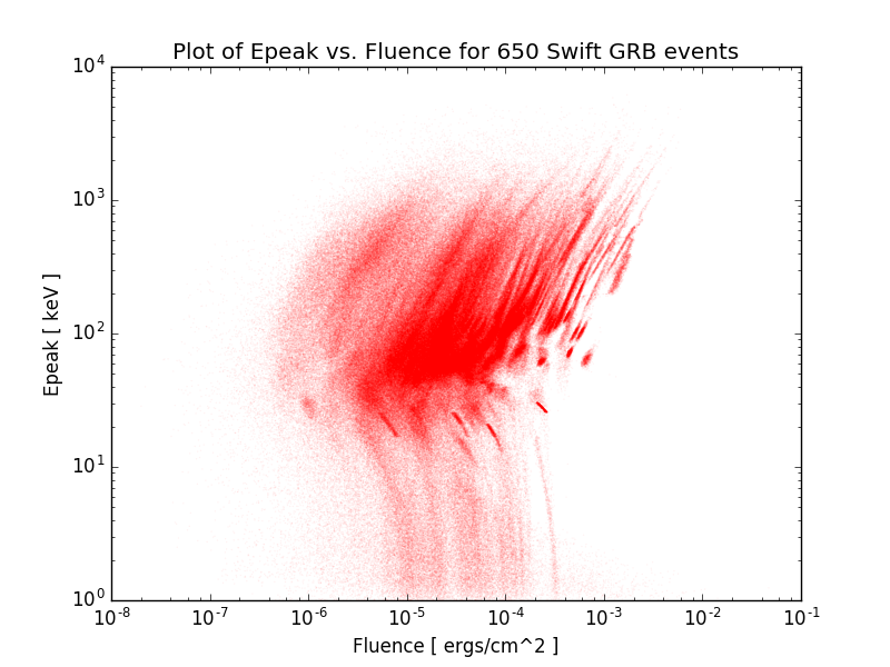
(C) Now write a third function, that reads all of these files in your directory, one by one, as numpy arrays, and plots the content of all of them together, on a single scatter plot like the following,
To achieve this goal, your function should start like the following,
def plotBatFiles(inPath,figFile):
    import os
    import numpy as np, os
    import matplotlib.pyplot as plt
    ax = plt.gca()  # generate a plot handle
    ax.set_xlabel('Fluence [ ergs/cm^2 ]') # set X axis title
    ax.set_ylabel('Epeak [ keV ]')  # set Y axis title
    ax.axis([1.0e-8, 1.0e-1, 1.0, 1.0e4]) # set axix limits [xmin, xmax, ymin, ymax]
    plt.hold('on')  # add all data files to the same plot
    counter = 0     # counts the number of events
where inPath and figFile are the path to the directory containing the files, and the name and path to the output figure file. You will have to use os.listdir(inPath) to get a list of all files in your input directory. Then loop over this list of files, and use only those that end with ep_flu.txt because that’s how you saved those files, e.g.,
for file in os.listdir(inPath):
        if file.endswith("ep_flu.txt"):
            # rest of your code ...
But now, you have to also make sure that your input data does indeed contain some numerical data, because some files do contain anything, although they exist, like this file: ``. To do so, you will have to perform a test on the content of file, once you read it as numpy array, like the following,
            data = np.loadtxt(os.path.join(inPath, file), skiprows=1)
            if data.size!=0 and all(data[:,1]<0.0):
                # then plot data
the condition all(data[:,1]<0.0) is rather technical. It makes sure that all values are positive on the second column. Once you have done all these checks, you have to do one final manipulation of data, that is, the data in these files on the second column is actually the log of data, so have to get the exp() value to plot it (because plot is log-log). To do so you can use,
data[:,1] = np.exp(data[:,1])
and then finally,
ax.scatter(data[:,1],data[:,0],s=1,alpha=0.05,c='r',edgecolors='none')
which will add the data for the current file to the plot. At the end, you will have to set a title for your plot as well, and save your plot,
    ax.set_title('Plot of Epeak vs. Fluence for {} Swift GRB events'.format(counter))
    plt.savefig(figFile)
Note that the variable counter contains the total number of events for which the text files exists on the website, and the file contained some data (i.e., was not empty).
Question: What does alpha=0.05 and s=1 do in the following scatter plot command? (Vary their values to see what happens)
2. Simulating a fun Monte Carlo game. Suppose you’re on a game show, and you’re given the choice of three doors:

Behind one door is a car; behind the two others, goats. You pick a door, say No. 1, and the host of the show opens another door, say No. 3, which has a goat.

He then says to you, “Do you want to pick door No. 2?”.
Question: What would you do?
Is it to your advantage to switch your choice from door 1 to door 2? Is it to your advantage, in the long run, for a large number of game tries, to switch to the other door?
Now whatever your answer is, I want you to check/prove your answer by a Monte Carlo simulation of this problem. Make a plot of your simulation for $ngames=100000$ repeat of this game, that shows, in the long run, on average, what is the probability of winning this game if you switch your choice, and what is the probability of winning, if you do not switch to the other door.