This lecture discusses some further important topics in Python IO, the use of random numbers and Monte Carlo simulations, as well as methods of integrating Python codes with codes from other programming languages, in particular, the use of Python as a wrapper for highly efficient, fast, low-level codes written in Fortran and C.

More on IO in Python

There are a few topics and methods of input/output (IO) in Python that we have not discussed yet, such as reading data from special data files, or web pages. Such problems, happen almost daily in a scientific research career, even in High Performance Computing, and Python’s capability to easily handle such IO problems is indeed one of the main reasons for Python’s popularity.

Reading data from special data files

It will happen quite often in your research that you will need to read data from a spreadsheet data file, most importantly *.csv and Microsoft Excel files (e.g., *.xls data files), or also frequently, from an *.xml data file. There are many ways and Python libraries to read such files. For Excel files, the task can be a bit complex, since Excel files can contain multiple sheets. A good starting point might be this webpage, also Pandas module.

For CSV files, Python standard library has a solution. Suppose you want to read this CSV file. A Python solution would be the following,

import csv
with open('jec_pdb_r4s.csv','r') as myfile:
    for counter, row in enumerate(csv.reader(myfile)):
        print(row)
        if counter>10: break

['pdb', 'pdb_id', 'chain', 'site', 'zr4s_JTT', 'r4s_JTT', 'zr4s_JC', 'r4s_JC']
['132L_A', '132L', 'A', '2', '-0.3133', '1.02', '0.04475', '1.188']
['132L_A', '132L', 'A', '3', '0.8385', '1.955', '0.2036', '1.311']
['132L_A', '132L', 'A', '4', '2.093', '2.973', '1.451', '2.272']
['132L_A', '132L', 'A', '5', '-0.8878', '0.5537', '-0.7985', '0.5382']
['132L_A', '132L', 'A', '6', '-1.443', '0.1028', '-1.426', '0.05416']
['132L_A', '132L', 'A', '7', '-0.1195', '1.177', '-0.07917', '1.093']
['132L_A', '132L', 'A', '8', '-0.7236', '0.6869', '-0.8997', '0.4602']
['132L_A', '132L', 'A', '9', '-1.107', '0.3755', '-0.8971', '0.4622']
['132L_A', '132L', 'A', '10', '0.7076', '1.848', '0.7369', '1.722']
['132L_A', '132L', 'A', '11', '0.9573', '2.051', '0.8809', '1.833']
['132L_A', '132L', 'A', '12', '-0.8315', '0.5993', '-0.9243', '0.4413']

Note how I have used Python enumerate() function to control the number of lines that is read from the file (The file contains more than 70000 lines of data!).

Similarly, if you wanted to write a CSV file, you can use csv.writer() method,

with open('jec_pdb_r4s.csv','r') as infile, open('jec_out.csv', 'w') as outfile:
    for counter, row in enumerate(csv.reader(infile)):
        csv.writer(outfile).writerow(row)
        if counter>10: break

The output of the code is this file (If you run this code on Windows machines, you will probably get an extra empty line between each row in the csv file).

For *.xml files, Python standard library has a package ElementTree, which you can use for both parsing and writing xml data files.

Reading data from web

Nowadays, a lot of data repositories are available online publicly, and you may encounter problems that need to parse data from an online repository. For many of the most famous repositories, such as the Protein databank, excellent python packages have been written that automate the process of fetching data from online pages or repositories (e.g., Biopython).

Nevertheless you may need at some point in your research or career to read data from a web address. Most often, the online data is contained in a html file, like the content of the about page for this course, for example, which has the address: https://www.cdslab.org/ECL2017S/about. Suppose you wanted to extract the content of this page. A simple solution would be the following via Python’s standard urllib module,

import urllib.request as ur
myurl = 'https://www.cdslab.org/ECL2017S/about'
with ur.urlopen(myurl) as webfile:
    webcontent = [line.decode("utf-8") for line in webfile.readlines()]

Now the variable webcontent is a list, whose elements are each row in the html file for this page.

webcontent[0:10]

['<!DOCTYPE html>\n',
'<html>\n',
'<head>\n',
'<meta charset="utf-8">\n',
'<title>COE 111L - SPRING 2017</title>\n',
'<meta name="description" content="Engineering Computation Lab">\n',
'<meta name="keywords" content="Amir, Shahmoradi, Instructor">\n',
'\n',
'<!-- Twitter Cards -->\n',
'<meta name="twitter:card" content="summary_large_image">\n']

Note that the content of the file is read in byte format. Therefore, to convert it to string, one has to apply .decode("utf-8") on each line. Similar to opening a file on harddisk, one can also use .read() and .readline() methods to read the contant of the web address. Alternatively, one could also save the entire content of the web address, in a single file locally,

import urllib.request as ur
myurl = 'https://www.cdslab.org/ECL2017S/about'
ur.urlretrieve(myurl, filename='about.html')

This will output this file in your current working diretory of Python.

Now, the file that we imported from the web does not contains any scientific data. But, in the homework you will see a real-world scientific example and value of Python’s ability to parse the content of web pages.

Writing data in HTML (web) format

Doing research at a professional level requires reporting the results professionally as well. That is, the results of the project, including the final report itself have to be auto-generated and reproducile as much as possible, and reachable to the widest audience (which nowadays means, availibility on the world-wide web).

Suppose you have worked on your final project for this course, which has resulted in several figures, that you wanted to put them all together on a single webpage in your repository on Github, together with some information about each figure. Let’s say the figures are figure 1 , figure 2 , figure 3 , figure 4 , figure 5 , figure 6 , figure 7. Now, since these figures represent the time evolution of the growth of the tumor, you would wnat to write a code that automatically generates an HTML (or Markdown) files, which contains the correct HTML code for adding these figures in your page for the project. You could for example write the following Python code to achieve this goal,

with open('SampleProjectReport.html', 'w') as html:
    html.write('<HTML><BODY BGCOLOR="white">\n')
    html.write('<H1>Sample Semester Project: Tumor growth modeling</H1><br> \n')
    html.write('<H2>Each of following subplots figure represents the stage of the growth of tumor at the specified date in the figure title.</H2><br><br> \n')

    time = [10.0,12.0,14.0,15.0,16.0,18.0,20.0]
    nfig = 7
    figReposPrefix = 'https://www.cdslab.org/ECL2017S/exam/2/figures/tvccZSliceSubplotWithXYlab_rad_00gy_'
    for ifig in range(1,nfig+1):
        html.write( '<img src="{}{:d}_t{:.1f}.png" width="900px"><br><br>\n'.format(figReposPrefix,ifig,time[ifig-1]) )
    html.write('<H2>Conclusions:</H2>\n')
    html.write('<p>Chances of survival for this rat are virtually zero.</p><br>\n')
    html.write('</BODY></HTML>\n')

This code will generate an HTML file, which you can view in browser here.

Random numbers in Python

One of the most important topics in todays’s science and computer simulation is random number generation and Monte Carlo simulation methods. In the simplest scenario for your research, you may need to generate a sequence of uniformly distributed random numbers in Python. There are several approaches to handle such random number generation problems in Python. Here is one, via Python’s standard random module:

In [43]: import random as rnd

In [44]: rnd.random()   # generates a random number in the half open interval [0,1)
Out[44]: 0.012519922307372311

In [45]: rnd.
rnd.BPF             rnd.Random          rnd.betavariate     rnd.gauss           rnd.normalvariate   rnd.randrange       rnd.shuffle         rnd.weibullvariate
rnd.LOG4            rnd.SG_MAGICCONST   rnd.choice          rnd.getrandbits     rnd.paretovariate   rnd.sample          rnd.triangular
rnd.NV_MAGICCONST   rnd.SystemRandom    rnd.expovariate     rnd.getstate        rnd.randint         rnd.seed            rnd.uniform
rnd.RECIP_BPF       rnd.TWOPI           rnd.gammavariate    rnd.lognormvariate  rnd.random          rnd.setstate        rnd.vonmisesvariate

As you see in the list of available methods in random, you can generate random numbers from a wide variaty of univariate probability distributions, e.g.,

In [46]: rnd.betavariate(0.5,0.5)   # Beta variate with the input parameters
Out[46]: 0.9281984408820623

In [54]: rnd.expovariate(1)         # random variable from exponential distribution with mean 1.
Out[54]: 2.546912414260747

In [55]: rnd.gammavariate(1,1)      # random variable from gamma distribution with parameters 1,1.
Out[55]: 0.5364897808236537

Recall that if you needed help on a method or function in Python, you could use help(),

In [61]: help(rnd.weibullvariate)
Help on method weibullvariate in module random:

weibullvariate(alpha, beta) method of random.Random instance
    Weibull distribution.

    alpha is the scale parameter and beta is the shape parameter.

To generate float random numbers between the given input bounds,

In [64]: rnd.uniform(50,100)    # generate a random float between 50 and 100
Out[64]: 65.59688328558263

ATTENTION:

Alwasy make sure you import modules with unique names, as different modules with similar component names may overwrite each other. For example import random followed by from numpy import * wil cause the random module to be overwritten by numpy.random module.

Also pay attention to sublte differences between similar functions, with the same names, but in different modules. For example,

import numpy as np
np.random.randint(1,6,1)

will draw a random integer from the interval $[1,6)$ excluding the value $6$ (the third input, $1$, indicates how many numbers has to be drawn randomly by the function). However,

import random as rnd
rnd.randint(1,6)

will draw a random integer form the interval $[1,6]$. Also note that randint() from module random is a scalar function, whereas the numpy’s version is vectorized.

The deterministic aspect of randomness in Python

There is a truth about random numbers and random number generators and algorithms, not only in Python, but in all programming languages, and that is, true random numbers do not exist in the world of programming. What we call a seuqence of random numbers, is simply a sequence of numbers that we, the user, to the best of our knowledge, don’t know how it was generated, and therefore, the sequence looks random to us, bu not the to the developer of the algorithm!. To prove this, type the following code in a Python session,

In [13]: import numpy as np

In [14]: np.random.seed(42)

In [15]: np.random.randint(1,6,6)
Out[15]: array([4, 5, 3, 5, 5, 2])

In [16]: np.random.randint(1,6,6)
Out[16]: array([3, 3, 3, 5, 4, 3])

In [17]: np.random.seed(42)

In [18]: np.random.randint(1,6,6)
Out[18]: array([4, 5, 3, 5, 5, 2])

You notice that everytime the random function is called, it generates a new sequence of random numbers, apparently completely random. But as soon as the function np.random.seed(42) is called, it appears that the random number generator also restarts from the beginning, generating the same sequence of random numbers as it did before.

You can even test the same code on a different computer, and as long as you set the seed of the random number generator to a specific value (here 42), np.random.seed(42), you will the same sequence of random numbers. So afterall, random numbers are not random at all, as they can be generated detrerministically, however, they mimic the behavior of true random numbers. The ability to set the seed for a random number generator is actually very useful, since it enables us to replicate the work of a code, exactly it has been done in the past. In particular, this is very useful for code debugging. However, beware of cases were you need to get a different result, everytime you run the code. If you set the random seed of the random generator to to a fixed value, right at the beginning of the code, you will never get a random behavior.

Drawing a random element from a list

Suppose you have the following list,

import numpy as np
mylist = np.linspace(0,100,51)

mylist

array([   0.,    2.,    4.,    6.,    8.,   10.,   12.,   14.,   16.,
         18.,   20.,   22.,   24.,   26.,   28.,   30.,   32.,   34.,
         36.,   38.,   40.,   42.,   44.,   46.,   48.,   50.,   52.,
         54.,   56.,   58.,   60.,   62.,   64.,   66.,   68.,   70.,
         72.,   74.,   76.,   78.,   80.,   82.,   84.,   86.,   88.,
         90.,   92.,   94.,   96.,   98.,  100.])

and now you wanted to draw a random element from the above list. You could do,

import random as rnd
rnd.choice(mylist)

80.0 

This will give a random element from the list. You could also generate a random shuffling of the list by,

import random as rnd
rnd.shuffle(mylist)
mylist

array([  98.,   12.,   76.,   60.,   46.,   22.,   24.,   92.,   66.,
         16.,    6.,   34.,   14.,    8.,   18.,   50.,   30.,   74.,
          4.,    2.,   38.,   90.,   70.,   56.,   94.,   80.,   32.,
         20.,   10.,   44.,   72.,   84.,    0.,   78.,  100.,   88.,
         86.,   96.,   48.,   52.,   62.,   64.,   26.,   36.,   40.,
         54.,   68.,   58.,   82.,   42.,   28.])

Summary of some important random functions in Python

As you may have noticed, since none of the random functions are builtin, things can get really confusing very easily, by simply mixing numpy’s random mdule with Python’s random module. The following helps to clarify some of the most important differences between these two modules.

Table 1: Some useful functions and their functionalities in random and numpy modules

Purpose	random module	numpy.random module
random uniform numbers in $[0,1)$	random()	random(N) (vectorized)
random uniform numbers in $[a,b)$	uniform(a,b)	uniform(a,b,N) (vectorized)
random integers in $[a,b]$	randint(a,b)	randint(a,b+1,N) (vectorized) random_integers(a,b+1,N) (vectorized)
random Gaussian deviate with parameters $[\mu, \sigma]=[m,s]$	gauss(m,s)	normal(m,s,N) (vectorized)
setting random number generator seed $i$	seed(i)	seed(i)
shuffling list mylist	shuffle(mylist)	shuffle(mylist)
choose a random element from mylist	choice(mylist)	--

Monte Carlo simulations

A Monte Carlo simulation is basically any simulation problem that somehow involves random numbers. Let’s start with an example of throwing a die repeatedly for N times. We can simulate the process of throwing a die by the following python code,

def throwFairDie():
    import random as rnd
    return rnd.randint(1, 6)

Now, each time the function is called, it returns a random value for one throw of a virtual die,

In [7]: throwFairDie()
Out[7]: 6

In [8]: throwFairDie()
Out[8]: 1

In [9]: throwFairDie()
Out[9]: 4

In [10]: throwFairDie()
Out[10]: 1

This is likely one of the simplest examples of Monte Carlo simulations. Now suppose we wanted to make sure that the die is fair, meaning that each number (out of 6 possibilities) only appears with a frequency of $1/6$ over many throws of the die. To test this hypothesis, we could write the following code,

import numpy as np

def throwFairDie():
    import random as rnd
    return rnd.randint(1, 6)

def getMeanDieValue(n=10000):
    meanDieValue = np.zeros((n,6),dtype=np.double)
    randomThrow = throwFairDie() - 1        # assign the first value to the above array
    meanDieValue[0,randomThrow] = 1.0 / 1.0 # one try so far, one success for the die value that is obtained.
    for i in range(1,n):
        randomThrow = throwFairDie() - 1
        meanDieValue[i,randomThrow] = 1.0   # add one success for the value obtained
        meanDieValue[i,:] += meanDieValue[i-1,:]    # combine the recent success with the total number of successes from previous tries.
        meanDieValue[i-1,:] /= np.double(i)  # Now normalize the values form the last try to the total number of tries.
    meanDieValue[-1:,:] /= np.double(n)  # Now normalize the very last try to the total number of tries.
    return meanDieValue

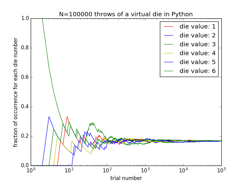
What this function does, is that it throws a die for given input number of times (n=10000 by default if not given as input), and then calculates for each new try, how many times each of the die values have occurred so far, and then finally outputs all the result as numpy double array, each row of which contains the number of successes for each of the 6 die values. Normally, if the die is fair, you would expect that with more tries, the average number of successes for each try would converge more and more to the canonical value $1/6\sim0.1667$. We can test this, by calling the function with a large number of tries, and checking the values in the last row of the output array,

print( getMeanDieValue()[-1:,:] )

[[ 0.1645  0.1668  0.1683  0.1664  0.169   0.165 ]]

print( getMeanDieValue(n=100000)[-1:,:] )

[[ 0.16488  0.1665   0.16635  0.16841  0.1661   0.16776]]

A better approach would be plot the output as a function of the number of tries, and see if the results for each of possible die outcomes do indeed converge to the canonical value or not.

import numpy as np
import matplotlib.pyplot as plt

nDieValues = 6 # 6 possible values for a die throw
nTrial = 100000 # total number of die throws
meanDieValues = getMeanDieValue(n=nTrial)

fig1 = plt.figure()
trial = np.linspace( 1 , nTrial+1 , nTrial )
lineTypes = ['r-','b-','g-','y-','b-','g-']
for i in range( nDieValues ) :
    plt.semilogx( trial[:] \
            , meanDieValues[:,i] \
            , lineTypes[i] \
            ) # plot with color red, as line
    plt.hold('on')
plt.xlabel('trial number')
plt.ylabel('fraction of occurrence for each die number')
plt.legend(['die value: '+str(i) for i in range(1,7) ])
plt.axis([1, nTrial , 0.0, 1.0]) # [xmin, xmax, ymin, ymax]
plt.title('N={} throws of a virtual die in Python'.format(nTrial))
plt.savefig('diceThrowsN{}.png'.format(nTrial))
plt.show()

You can see the output of the above code in the following figure,

Python wrappers and interfaces

Python is a very convenient language for implementing scientific computations as the code can be made very close to the mathematical algorithms. However, the execution speed of the code is significantly lower than what can be obtained by programming in languages such as Fortran, C, or C++. For example see the following performance comparisons and tests in NASA modeling guru webpage. As you can see there, the performance of Python code can be significantly lower, up to 500 times and more, compared to compiled languages such as Fortran and C. These languages compile the program to machine language, which enables the computing resources to be utilized with very high efficiency. Knowing the performance hit in Python, the scientific programming paradigm in Python is to write compute-intensive parts of the code in lower level languages such as Fortran or C, and use Python as wrapper and glue between lower level codes and as a handy tool for high-level tasks.

Python was initially designed for being integrated with C. This feature has spawned the development of several techniques and tools for calling compiled languages from Python, allowing us to relatively easily reuse fast and well-tested scientific libraries in Fortran, C, or C++ from Python, or migrate slow Python code to compiled languages. It often turns out that only smaller parts of the code, usually for loops doing heavy numerical computations, suffer from low speed and can benefit from being implemented in Fortran, C, or C++.

There are already several Python wrappers developed for integrating Python with other programming language codes. Most prominent examples include F2PY for Fortran and C codes, SWIG for C, C++, Perl, Java, and many others, Cython for C, Jython for Java, and several others.

The usage of some of these wrappers can be tricky and requires some work and good familiarity with the wrapper. This is in particular true about SWIG, which involves a significant amount of manual modifications to the interfaces, compared to F2PY, for example. At the moment, F2PY only works with Python 2.x standard.

There is also a Python module pymat developed for direct interaction of Python code with MATLAB.