This is the solution to Homework 4: Problems - loops, IO.
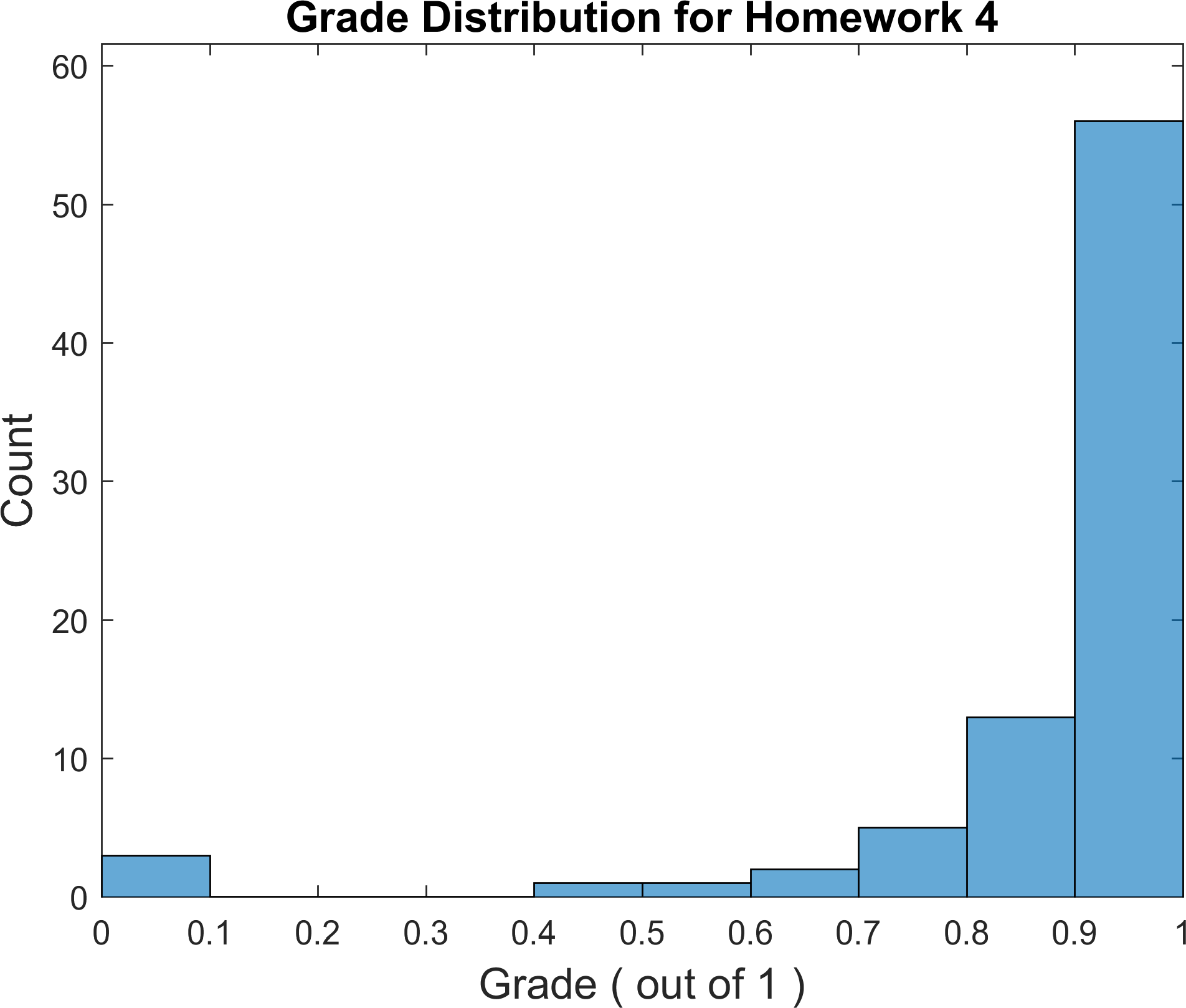
The following figure illustrates the grade distribution for this homework.
♣ Due Date: Monday Nov 13, 2017 9:00 AM. This homework aims at giving you some experience with MATLAB for-loops and while-loops as well as input/output functionalities in MATLAB.
1. The while-loop implementation of a for-loop. Consider the following two vectors of temperatures in Celsius degrees to Fahrenheit, using a for-loop and then prints them on screen.
Cdegrees = [-20, -15, -10, -5, 0, 5, 10, 15, 20, 25, 30, 35, 40]
Fdegrees = [-20, -15, -5, 0, 10, 15, 30, 35, 40]
(A) Write a function that takes an input vector of temperatures, and a string which is either 'F2C' or C2F. Then, converts the input temperature vector from Fahrenheit to Celsius if the input string is 'F2C', otherwise converts the input temperature vector from Celsius to Fahrenheit if the input string is 'C2F', otherwise outputs an error message and aborts the program.
(A) Write this function using while-loop construct (you can name the function convertTempFor.m).
(B) Write this function using for-loop construct (you can name the function convertTempWhile.m).
(C) Write this function using vectorization concept (you can name the function convertTempVec.m).
Here are some example calls to these functions,
InVec = [-20, -15, -10, -5, 0, 5, 10, 15, 20, 25, 30, 35, 40];
>> convertTempFor(InVec,'C2F')
ans =
    -4     5    14    23    32    41    50    59    68    77    86    95   104
>> convertTempWhile(InVec,'C2F')
ans =
    -4     5    14    23    32    41    50    59    68    77    86    95   104
>> convertTempVec(InVec,'C2F')
ans =
    -4     5    14    23    32    41    50    59    68    77    86    95   104
Answer:
Here are the three convertTempFor.m, convertTempWhile.m, and convertTempVec.m functions.
2. Use MATLAB built-in timing functions to measure the performance of three functions you wrote in question 1 above.
Answer:
Here is one way (timing.m script) to time the functions. Here is a test result:
>> timing
Timing for convertTempVec: 0.038723 seconds.
Timing for convertTempFor: 0.03936 seconds.
Timing for convertTempWhile: 0.18011 seconds.
3. Consider the following nested cell vector,
List = { {'M','A','T','L','A','B'}, {' '}, {'i','s'}, {' '}, {'a'}, {' '}, {'s','t','r','a','n','g','e'}, {', '}, {'b','u','t',' '}, {'p','o','p','u','l','a','r'}, {' '}, {'p','r','o','g','r','a','m','m','i','n','g',' ','l','a','n','g','u','a','g','e'} };
Write a MATLAB script extractLetter.m that uses for-loop to extract all the letters in the variable list and finally prints them all as a single string like the following,
>> extractLetter
MATLAB is a strange, but popular programming language
Answer:
Here is an example implementation.
4. The significant impact of round-off errors in numerical computation. Consider the following program,
formatSpec = 'With %d sqrt, then %d times ^2 operations, the number %.16f becomes: %.16f \n'; % the string format for fprintf function
for n = 1:60
    r_original = 2.0;
    r = r_original;
    for i = 1:n
        r = sqrt(r);
    end
    for i = 1:n
        r = r^2;
    end
    fprintf(formatSpec,n,n,r_original,r);
end
Explain what this code does. Then run the code, and explain why do you see the behavior observed. In particular, why do you not recover the original value $2.0$ after many repetitions of the same forward and reverse task of taking square root and squaring the result?
Answer:
This code (roundoff.m) will yield the following output:
>> roundoff
With 1 sqrt, then 1 times ^2 operations, the number 2.0000000000000000 becomes: 2.0000000000000004
With 2 sqrt, then 2 times ^2 operations, the number 2.0000000000000000 becomes: 1.9999999999999996
With 3 sqrt, then 3 times ^2 operations, the number 2.0000000000000000 becomes: 1.9999999999999996
With 4 sqrt, then 4 times ^2 operations, the number 2.0000000000000000 becomes: 1.9999999999999964
With 5 sqrt, then 5 times ^2 operations, the number 2.0000000000000000 becomes: 1.9999999999999964
With 6 sqrt, then 6 times ^2 operations, the number 2.0000000000000000 becomes: 1.9999999999999964
With 7 sqrt, then 7 times ^2 operations, the number 2.0000000000000000 becomes: 1.9999999999999714
With 8 sqrt, then 8 times ^2 operations, the number 2.0000000000000000 becomes: 2.0000000000000235
With 9 sqrt, then 9 times ^2 operations, the number 2.0000000000000000 becomes: 2.0000000000000235
With 10 sqrt, then 10 times ^2 operations, the number 2.0000000000000000 becomes: 2.0000000000000235
With 11 sqrt, then 11 times ^2 operations, the number 2.0000000000000000 becomes: 2.0000000000000235
With 12 sqrt, then 12 times ^2 operations, the number 2.0000000000000000 becomes: 1.9999999999991336
With 13 sqrt, then 13 times ^2 operations, the number 2.0000000000000000 becomes: 1.9999999999973292
With 14 sqrt, then 14 times ^2 operations, the number 2.0000000000000000 becomes: 1.9999999999973292
With 15 sqrt, then 15 times ^2 operations, the number 2.0000000000000000 becomes: 1.9999999999973292
With 16 sqrt, then 16 times ^2 operations, the number 2.0000000000000000 becomes: 2.0000000000117746
With 17 sqrt, then 17 times ^2 operations, the number 2.0000000000000000 becomes: 2.0000000000408580
With 18 sqrt, then 18 times ^2 operations, the number 2.0000000000000000 becomes: 2.0000000000408580
With 19 sqrt, then 19 times ^2 operations, the number 2.0000000000000000 becomes: 2.0000000001573586
With 20 sqrt, then 20 times ^2 operations, the number 2.0000000000000000 becomes: 2.0000000001573586
With 21 sqrt, then 21 times ^2 operations, the number 2.0000000000000000 becomes: 2.0000000001573586
With 22 sqrt, then 22 times ^2 operations, the number 2.0000000000000000 becomes: 2.0000000010885857
With 23 sqrt, then 23 times ^2 operations, the number 2.0000000000000000 becomes: 2.0000000029511749
With 24 sqrt, then 24 times ^2 operations, the number 2.0000000000000000 becomes: 2.0000000066771721
With 25 sqrt, then 25 times ^2 operations, the number 2.0000000000000000 becomes: 2.0000000066771721
With 26 sqrt, then 26 times ^2 operations, the number 2.0000000000000000 becomes: 1.9999999917775542
With 27 sqrt, then 27 times ^2 operations, the number 2.0000000000000000 becomes: 1.9999999917775542
With 28 sqrt, then 28 times ^2 operations, the number 2.0000000000000000 becomes: 1.9999999917775542
With 29 sqrt, then 29 times ^2 operations, the number 2.0000000000000000 becomes: 1.9999999917775542
With 30 sqrt, then 30 times ^2 operations, the number 2.0000000000000000 becomes: 1.9999999917775542
With 31 sqrt, then 31 times ^2 operations, the number 2.0000000000000000 becomes: 1.9999999917775542
With 32 sqrt, then 32 times ^2 operations, the number 2.0000000000000000 becomes: 1.9999990380770896
With 33 sqrt, then 33 times ^2 operations, the number 2.0000000000000000 becomes: 1.9999971307544144
With 34 sqrt, then 34 times ^2 operations, the number 2.0000000000000000 becomes: 1.9999971307544144
With 35 sqrt, then 35 times ^2 operations, the number 2.0000000000000000 becomes: 1.9999971307544144
With 36 sqrt, then 36 times ^2 operations, the number 2.0000000000000000 becomes: 1.9999971307544144
With 37 sqrt, then 37 times ^2 operations, the number 2.0000000000000000 becomes: 1.9999971307544144
With 38 sqrt, then 38 times ^2 operations, the number 2.0000000000000000 becomes: 1.9999360966436217
With 39 sqrt, then 39 times ^2 operations, the number 2.0000000000000000 becomes: 1.9999360966436217
With 40 sqrt, then 40 times ^2 operations, the number 2.0000000000000000 becomes: 1.9999360966436217
With 41 sqrt, then 41 times ^2 operations, the number 2.0000000000000000 becomes: 1.9994478907329654
With 42 sqrt, then 42 times ^2 operations, the number 2.0000000000000000 becomes: 1.9984718365144798
With 43 sqrt, then 43 times ^2 operations, the number 2.0000000000000000 becomes: 1.9965211562778555
With 44 sqrt, then 44 times ^2 operations, the number 2.0000000000000000 becomes: 1.9965211562778555
With 45 sqrt, then 45 times ^2 operations, the number 2.0000000000000000 becomes: 1.9887374575497223
With 46 sqrt, then 46 times ^2 operations, the number 2.0000000000000000 becomes: 1.9887374575497223
With 47 sqrt, then 47 times ^2 operations, the number 2.0000000000000000 becomes: 1.9887374575497223
With 48 sqrt, then 48 times ^2 operations, the number 2.0000000000000000 becomes: 1.9887374575497223
With 49 sqrt, then 49 times ^2 operations, the number 2.0000000000000000 becomes: 1.8682459487159784
With 50 sqrt, then 50 times ^2 operations, the number 2.0000000000000000 becomes: 1.6487212645509468
With 51 sqrt, then 51 times ^2 operations, the number 2.0000000000000000 becomes: 1.6487212645509468
With 52 sqrt, then 52 times ^2 operations, the number 2.0000000000000000 becomes: 1.0000000000000000
With 53 sqrt, then 53 times ^2 operations, the number 2.0000000000000000 becomes: 1.0000000000000000
With 54 sqrt, then 54 times ^2 operations, the number 2.0000000000000000 becomes: 1.0000000000000000
With 55 sqrt, then 55 times ^2 operations, the number 2.0000000000000000 becomes: 1.0000000000000000
With 56 sqrt, then 56 times ^2 operations, the number 2.0000000000000000 becomes: 1.0000000000000000
With 57 sqrt, then 57 times ^2 operations, the number 2.0000000000000000 becomes: 1.0000000000000000
With 58 sqrt, then 58 times ^2 operations, the number 2.0000000000000000 becomes: 1.0000000000000000
With 59 sqrt, then 59 times ^2 operations, the number 2.0000000000000000 becomes: 1.0000000000000000
With 60 sqrt, then 60 times ^2 operations, the number 2.0000000000000000 becomes: 1.0000000000000000
What is happening is that, 1 is returned for n >= 52 as square root of 2, that is, after 52 times square-root operation, the degree of accuracy required for representing the result goes beyond the degree of accuracy available in a MATLAB double precision number. Consequently, the later squaring operation on 1.00000000000000 will leave the number unchanged and therefore, 2 is not recovered.
5. Consider the following code,
eps = 1.0;
while 1.0 ~= 1.0 + eps
    disp(num2str(eps));
    eps = eps / 2.0;
end
disp(['final eps:', num2str(eps)]);
Explain what the code is doing. Run the code and observe the output. How could 1.0 ~= 1.0 + eps be false?!
Answer:
Here is the output of the code,
>> epsError
eps: 1
eps: 0.5
eps: 0.25
eps: 0.125
eps: 0.0625
eps: 0.03125
eps: 0.015625
eps: 0.0078125
eps: 0.0039063
eps: 0.0019531
eps: 0.00097656
eps: 0.00048828
eps: 0.00024414
eps: 0.00012207
eps: 6.1035e-05
eps: 3.0518e-05
eps: 1.5259e-05
eps: 7.6294e-06
eps: 3.8147e-06
eps: 1.9073e-06
eps: 9.5367e-07
eps: 4.7684e-07
eps: 2.3842e-07
eps: 1.1921e-07
eps: 5.9605e-08
eps: 2.9802e-08
eps: 1.4901e-08
eps: 7.4506e-09
eps: 3.7253e-09
eps: 1.8626e-09
eps: 9.3132e-10
eps: 4.6566e-10
eps: 2.3283e-10
eps: 1.1642e-10
eps: 5.8208e-11
eps: 2.9104e-11
eps: 1.4552e-11
eps: 7.276e-12
eps: 3.638e-12
eps: 1.819e-12
eps: 9.0949e-13
eps: 4.5475e-13
eps: 2.2737e-13
eps: 1.1369e-13
eps: 5.6843e-14
eps: 2.8422e-14
eps: 1.4211e-14
eps: 7.1054e-15
eps: 3.5527e-15
eps: 1.7764e-15
eps: 8.8818e-16
eps: 4.4409e-16
eps: 2.2204e-16
final eps:1.1102e-16
What is happening is that after a certain number of divisions performed on the value of eps, the value goes beyond the highest float precision representable by Python standard ($0.0000000000000001$), and therefore the value of eps is eventually rounded to exact zero. The nonzero eps value computed above is called machine epsilon or machine zero and is an important parameter to know, since it can lead to disasters in your very important complex calculations.
6. Suppose you want to find the largest prime number that is smaller than a given input value by the user. Write a function named getLargestPrime that does so, using for-loop, break, and MATLAB’s intrinsic function isprime(). Here is a test,
>> getLargestPrime(123)
ans =
   113
Answer:
function integer = getLargestPrime(upper)
    if (upper<1)
        disp('input value cannot be less than 1. Goodbye!')
        return
    end
    for integer = upper:-1:1
        if isprime(integer)
            break
        end
    end
end
6. Consider the problem number 5 in HW 3, where we wrote a function named fib.m that used the idea of recursive functions to generate the Fibonacci numbers.
(A) Download this function fib() and modify it using MATLAB timeit() function such that it also returns the average runtime of getFib() nested function inside fib(), right after giving the requested Fibonacci number. For example, here is an output from such modified code:
>> fib
Please enter a non-negative integer or type stop: 10
	fib(10) = 55
	average runtime: 1.0083e-05 seconds
Please enter a non-negative integer or type stop: 15
	fib(15) = 610
	average runtime: 8.8884e-05 seconds
Please enter a non-negative integer or type stop: 20
	fib(20) = 6765
	average runtime: 0.00095559 seconds
Please enter a non-negative integer or type stop: 25
	fib(25) = 75025
	average runtime: 0.010311 seconds
Please enter a non-negative integer or type stop: 30
	fib(30) = 832040
	average runtime: 0.11575 seconds
Please enter a non-negative integer or type stop: 35
	fib(35) = 9227465
	average runtime: 1.2904 seconds
Please enter a non-negative integer or type stop: stop
(Note that you can use char(9) at the beginning of your disp() messages in order to add the tab character at the beginning of your message, just like the above example.)
(B) Now copy this function to a new MATLAB M-file named fibLoop.m. Also modify the name of the function fib() in this file fibLoop(). Modify the nested function getFib() inside of fibLoop() such that instead of recursive function calls, it uses a for-loop to find the requested Fibonacci number.
(C) Now time your new function fibLoop() for the same input integers as in the above example: $10,15,20,25,30,35$. How do the runtimes for fibLoop() compare with fib(). Which function is faster and more efficient: fib() or fibLoop()? Why is there such huge difference in the performance of the two functions?
Answer:
Here is an implementation of the modified fib() and modified fib().
>> fibLoop
Please enter a non-negative integer or type stop: 12
	fib(12) = 144
	average runtime: 4.3496e-06 seconds
Please enter a non-negative integer or type stop: 10
	fib(10) = 55
	average runtime: 4.5323e-06 seconds
Please enter a non-negative integer or type stop: 15
	fib(15) = 610
	average runtime: 4.5232e-06 seconds
Please enter a non-negative integer or type stop: 20
	fib(20) = 6765
	average runtime: 4.6357e-06 seconds
Please enter a non-negative integer or type stop: 25
	fib(25) = 75025
	average runtime: 4.6562e-06 seconds
Please enter a non-negative integer or type stop: 30
	fib(30) = 832040
	average runtime: 4.7624e-06 seconds
Please enter a non-negative integer or type stop: 35
	fib(35) = 9227465
	average runtime: 4.7889e-06 seconds
Please enter a non-negative integer or type stop: stop
As you see, the for-loop version of the function fibLoop() is far faster than the recursive function version fib(). The reason is that the recursive version is not well written and does a lot of redundant calculations. Ask me in class to explain for you why there is such a huge redundancy in this function calculations.
7. (A) Write two new MATLAB functions timeFib(n) and timeFibLoop(n) based on your MATLAB functions fib() and fibLoop() that you wrote in problem 6, such that both take an integer and output a structure whose fields are:
output.n
output.fib
output.runtime
Note that the function should take as input only an integer variable, so you need to modify your old codes to only check whether the input ~ischar(), and isreal() and n>=0 and round(n)==n. Here is an example output from the two functions,
>> timeFib(20)
ans =
          n: 20
        fib: 6765
    runtime: 9.6568e-04
>> timeFib('amir')
Error using timeFib (line 8)
The input argument is not a non-negative integer!
>> timeFibLoop(20)
ans =
          n: 20
        fib: 6765
    runtime: 4.4076e-06
>> timeFibLoop('amir')
Error using timeFibLoop (line 8)
The input argument is not a non-negative integer!
(B) Now write a script named writeFibResult.m that calls these two functions for a range of input $n={10,2,3,\ldots,35}$ values, and then write the output of these two functions in a formatted way in two files like these fibOutput.txt and fibLoopOutput.txt. You can use any of MATLAB IO methods to create the output file with any file extension you prefer: .txt, .csv, .xlsx, .tab, … .
Answer:
Here the two functions timeFib.m and timeFibLoop.m, and here is the script writeFibResult.m that creates the requested output file in the problem.