♣ Due Date: Friday Dec 1, 2017 11:59 PM. This homework aims at giving you some experience with data input/output methods in MATLAB as well as plotting graphs and Monte Carlo techniques.
1. Creating random 3-member student groups for the semester project Consider this csv data file which contains the names of all of the students in this course. Our goal here is to write a MATLAB script that reads all the names in this file, and then creates random triples of names to form student groups who would work collaboratively on the final semester project. To do so you will need MATLAB’s built-in function randperm() which creates random permutations of student IDs in the range 1-99. Once you create a random permutation, you will have to write a MATLAB for-loop which takes triples of integers from this vector of random permutations and puts the names corresponding to these IDs together in a cell array. Finally, this cell array of 33-by-3 elements could be written to an output Microsoft xlsx file, using MATLAB’s xlswrite() function. On output your script should yield an excel file like this one. To get the exact same order and triple of names, you will have to use rng(131313) at the beginning of your script in order to initialize the seed of MATLAB random number generator to 131313 so that the table can be regenerated every time you run your code.
2. Reading scientific data from web using MATLAB. Consider the following webpage address https://www.cdslab.org/ICP2017F/homework/5-problems/swift/bat_time_table.html. This is an data table (in HTML language) containing data from NASA’s Swift satellite. Each row in this table represents information about a Gamma-Ray Burst (GRB) detection that Swift has made in the past years. Now, corresponding to each of event IDs, there (might) exist files that contain some attributes of these events which we wish to plot and understand their behavior. For example, for the first event in this table, contains a data file which is hidden in a directory on this website here. For each event in this table, there is likely one such table hidden in this web directory.
Our goal in this question is to fetch all these files from the website, using MATLAB and save them locally in our own computer. Then read their contents one by one and plot the two columns of data in all of them together.
(A) Write a MATLAB script named fetchDataFromWeb.m that uses this web address: https://www.cdslab.org/ICP2017F/homework/5-problems/triggers.txt to read a list of all GRB events and then writes the entire table of triggers.txt to a local file with the same name on your device. For this purpose, you will need MATLAB built-in function webread().
(B) Now, add to your script another set of commands that uses the event IDs stored in this file, to generate the corresponding web addresses like: https://www.cdslab.org/ICP2017F/homework/5-problems/swift/GRB00745966_ep_flu.txt. Then it uses the generated web address to read the content of the page and store it in a local file on your device with the same name as it is stored on the webpage (for example, for the given webpage, the filename would be GRB00745966_ep_flu.txt). Note: Some of the web addresses for the given event IDs do not exist. Therefore, you should MATLAB’s try-catch construct to avoid runtime errors in your MATLAB code.
(C) Now write another MATLAB script named plotDatafromFile.m, that reads all of these files in your directory, one by one, using MATLAB readtable() function, and plots the content of all of them together, on a single scatter plot (using MATLAB function scatter()) like the following,
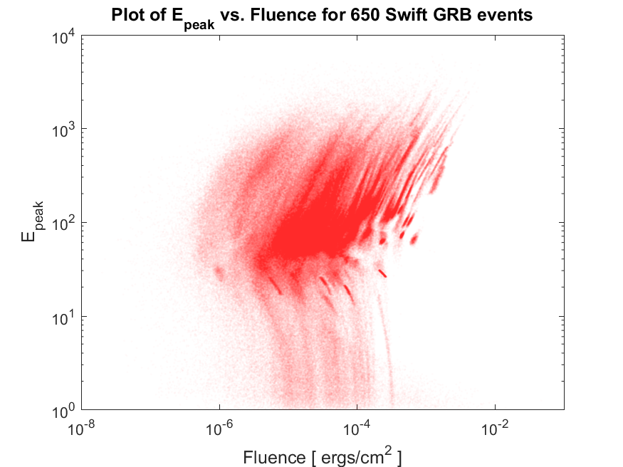
Note again that some the data files stored on your computer are empty and some others have useless data if data in the second column of the file is larger than 0. So you will have to write your script in such a way that it checks for non-emptiness of the file (that is, the file does indeed contain some numerical data) as well as the negativity of the values in the column of data in each file. For example, you could check for the negativity of the values using MATLAB function all(data[:,1]<0.0) assuming that data is the variable containing the information read from the file.
Once you have done all these checks, you have to do one final manipulation of data, that is, the data in these files on the second column is actually the log of data, so have to get the exp() value to plot it (because the plot in the figure above is a log-log plot and we want to exactly regenerate it). To do so you could simply use,
data[:,2] = exp(data[:,2]);
as soon as you read from the file, and then finally you make a scatter plot of all data using MATLAB scatter plot. At the end, you will have to set a title for your plot as well and label the axes of the plot, and save your plot using MATLAB’s built-in function saveas(). In order to find out how many files you have plotted in the figure, you will have to define a variable counter which increases by one unit, each time a new non-empty negative-second-column data file is read and plotted.
Hint: I strongly urge you to attend the next three lectures in order to answer this question.
3. Simulating a fun Monte Carlo game. Suppose you’re on a game show, and you’re given the choice of three doors:
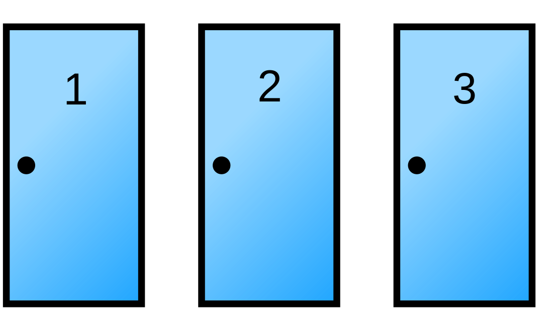
Behind one door is a car; behind the two others, goats. You pick a door, say No. 1, and the host of the show opens another door, say No. 3, which has a goat.

He then says to you, “Do you want to pick door No. 2?”.
Question: What would you do? Is it to your advantage to switch your choice from door 1 to door 2? Is it to your advantage, in the long run, for a large number of game tries, to switch to the other door?
Now whatever your answer is, I want you to check/prove your answer by a Monte Carlo simulation of this problem. Make a plot of your simulation for nExperiments=100000 repeat of this game, that shows, in the long run, on average, what is the probability of winning this game if you switch your choice, and what is the probability of winning, if you do not switch to the other door.
Hint: I strongly urge you to attend the lectures this week in order to get help for this question.
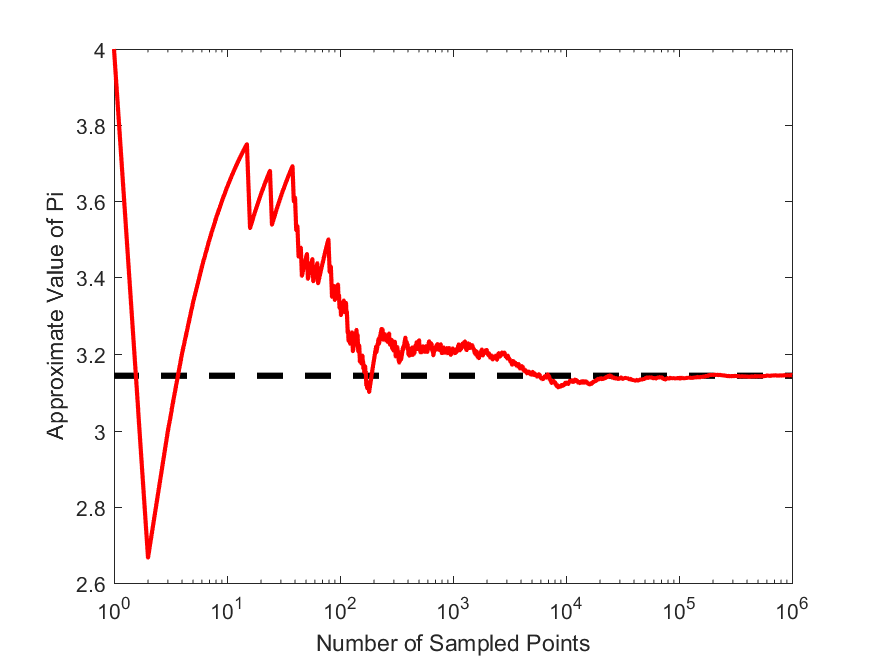
4. Monte Carlo approximation of the number $\pi$. Suppose we did not know the value of $\pi$ and we wanted to estimate its value using Monte Carlo methods. One practical approach is to draw a square of unit side, with its diagonal opposite corners extending from the coordinates origin $(0,0)$ to $(1,1)$. Now we try to simulate uniform random points from inside of this square by generating uniform random points along the $X$ and $Y$ axes, i.e., by generating two random uniform numbers (x,y) from the range $[0,1]$.
Now the generated random point $P$ has the coordinate $(x,y)$, so we can calculate its distance from the coordinate origin. Now suppose we also draw a quarter-circle inside of this square whose radius is unit and is centered at the origin $(0,0)$. The ratio of the area of this quarter-circle, $S_C$ to the area of the area of the square enclosing it, $S_S$ is,
This is because the area of the square of unit sides, is just 1. Therefore, if we can somehow measure the area of the quarter $S_C$, then we can use the following equation, to get an estimate of $\pi$,
In order to obtain, $S_C$, we are going to throw random points in the square, just as described above, and then find the fraction of points, $f=n_C/n_{\rm total}$, that fall inside this quarter-circle. This fraction is related to the area of the circle and square by the following equation,
Therefore, one can obtain an estimate of $\pi$ using this fraction,
Now, write a MATLAB script, that takes in the number of points to be simulated, and then calculates an approximate value for $\pi$ based on the Monte Carlo algorithm described above. Write a second function that plot the estimate of $\pi$ versus the number of points simulated, like the following,