This lecture explains the concept of for-loops and while-loops in MATLAB and different of types of it in MATLAB.

Lecture Videos

This video is created solely as reference for the attendants of ICP2017F course at UT Austin. If you did not attend this class, then you may not find this video useful.

Loops in MATLAB

Many programming algorithms require iteration, that is, the repetitive execution of a block of program statements. Similar to other programming languages, MATLAB also has built-in tools for iterative tasks in codes.

For-loop

The for-loop is among the most useful MATLAB constructs. The general syntax of for-loop is,

for variable = expression
    statements
end

Usually, expression is a vector of the form istart:stepSize:iend where fix((iend-istart)/stepSize+1) gives the number of iterations requested by the user, assuming iend>istart. The statements are the set of programming tasks that have to be repeated. For example consider a script named forLoop.m,

for index = istart:stepSize:iend
    disp(index);
end
disp( [ 'number of iterations: ', num2str( fix((iend-istart)/stepSize+1) ) ] );

>> istart = -2;
iend = 10;
stepSize = 3;
forLoop
    -2
     1
     4
     7
    10
number of iterations: 5

You can also iterate in reverse order,

>> istart = 10;
iend = -2;
stepSize = -3;
forLoop
    10
     7
     4
     1
    -2
number of iterations: 5

Breaking a for-loop immaturely

You can also use break inside a for-loop to get out of it, even before the for-loop finishes the full number of iterations. This is specially useful when you want to ensure if a condition has happened, and if so, then terminate the for-loop. For example,

for integer = 1:10
    disp(integer)
    if (integer==5)
        break
    end
end

 1
 2
 3
 4
 5

Exercise:
suppose you want to find the largest prime number that is smaller than a given input value by the user. Write a function that does so, using for-loop, break, and MATLAB’s intrinsic function isprime().

Answer:

function integer = getPrime(upper)
    if (upper<1)
        disp('input value cannot be less than 1. Goodbye!')
        return
    end
    for integer = upper:-1:1
        if isprime(integer)
            break
        end
    end
end

Continue statement within for-loops

To skip the rest of the instructions in a loop and begin the next iteration, you can use a continue statement. For example, the following code prints only integers that are primes,

for integer = 1:10
    if ~isprime(integer)
        continue
    end
    disp(['prime detected! ',num2str(integer)])
end

prime detected! 2
prime detected! 3
prime detected! 5
prime detected! 7

Iterating over vectors, matrices, and cell using for-loops

Note that the index of for-loop must not necessarily be an integer. Basically you can use the for-loop index to iterate over anything that is iterable in MATLAB. For example, consider the following,

a = [1,0,2,3,7,-1];
for index = a
    disp(class(index))
    disp(index)
end

The output of this script is,

double
    1
double
    0
double
    2
double
    3
double
    7
double
    -1

But, see what happens if we defined a as a matrix,

a = [1, 2, 3; 4, 5, 6; 7, 8, 9];
for index = a
    disp(class(index))
    disp(index)
end

double
    1
    4
    7
double
    2
    5
    8
double
    3
    6
    9

What is happening here? The answer is that, MATLAB is a column-wise programming language, just like Fortran, and unlike C, C++ and all of their descendants. MATLAB, by default, iterates over elements of row vectors. Therefore, when you use a matrix as the iterator in for-loops, MATLAB considers an entire column as the index of for-loop. The same is also true for other multidimensional arrays in MATLAB, for example cell arrays,

a = {1, 2, 3; 4, 5, 6; 7, 8, 9};
for index = a
    disp(class(index))
    disp(index)
end

cell
    [1]
    [4]
    [7]
cell
    [2]
    [5]
    [8]
cell
    [3]
    [6]
    [9]

Therefore, if you want to iterate over elements of a multidimensional matrix or array, you have to first reshape them using MATLAB’s built-in reshape() function to convert them to vector format, then iterating over them. For example,

a = {1, 2, 3; 4, 5, 6; 7, 8, 9};
a = reshape(a,[1,9]);
for index = a
    disp(class(index))
    disp(index)
end

cell
    [1]
cell
    [4]
cell
    [7]
cell
    [2]
cell
    [5]
cell
    [8]
cell
    [3]
cell
    [6]
cell
    [9]

Some general advice on for-loop index

• Avoid using $i$ and $j$ as index variables in for-loops. Note that i and j have special meanings in MATLAB, as described in previous lectures. They are used to define complex numbers. Using these variable names as indices in MATLAB for-loops, would overwrite the default meaning of these variables.
  
  
• Avoid assigning a value to the index variable within the loop statements. The for statement overrides any changes made to index within the loop.

While-loop

There is another iteration construct in MATLAB, called while-loop which has the following general syntax,

while expression
    statements
end

The statements within the while-loop are executed as long as expression is true. For example,

x = realmax();
while x>0
    xmin = x
    x = log(x)
end
xmin

xmin =
1.7977e+308
x =
709.7827
xmin =
709.7827
x =
    6.5650
xmin =
    6.5650
x =
    1.8817
xmin =
    1.8817
x =
    0.6322
xmin =
    0.6322
x =
-0.4585
xmin =
    0.6322

Note that, break and continue can be used in while-loops in the same fashion as they are used in for-loops, described above. The condition is evaluated before the body is executed, so it is possible to get zero iterations. It’s often a good idea to limit the number of repetitions to avoid infinite loops (as could happen above if x is infinite). This can be done in a number of ways, but the most common is to use break. For example,

n = 0;
while abs(x) > 1
    x = x/2;
    n = n+1;
    if n > 50, break, end
end

A break immediately jumps execution to the first statement after the loop. It’s good practice to include some diagnostic output or other indication that an abnormal loop exit has occurred once the code reach the break statement.

Exercise:
Write function getFac(n) using while-loop, that calculates the factorial of an input number n. For example,

>> getFac(4)
4! = 24

Some general advice on while-loops

• If you inadvertently create an infinite loop (that is, a loop that never ends on its own), stop execution of the loop by pressing Ctrl+C.
  
  
• If the conditional expression evaluates to a matrix, MATLAB evaluates the statements only if all elements in the matrix are true (nonzero). To execute statements if any element is true, wrap the expression in the any() function.
  
  
• To exit the loop, use a break statement as discussed above. To skip the rest of the instructions in the loop and begin the next iteration, use a continue statement.
  
  
• When nesting a number of while statements, each while statement requires an end keyword.

Vectorization in MATLAB

Experienced programmers who are concerned with producing compact and fast code try to avoid for loops wherever possible in their MATLAB codes. There is a reason for this: for-loops and while-loops have significant overhead in interpreted languages such as MATLAB and Python.

There is of course, a remedy for this inefficiency. Since MATLAB is a matrix language, many of the matrix-level operations and functions are carried out internally using compiled C, Fortran, or assembly codes and are therefore executed at near-optimum efficiency. This is true of the arithmetic operators *, +,-,\, / and of relational and logical operators. However, for loops may be executed relatively slowly—depending on what is inside the loop, MATLAB may or may not be able to optimize the loop. One of the most important tips for producing efficient M-files is to avoid for -loops in favor of vectorized constructs, that is, to convert for-loops into equivalent vector or matrix operations. Vectorization has important benefits beyond simply increasing speed of execution. It can lead to shorter and more readable MATLAB code. Furthermore, it expresses algorithms in terms of high-level constructs that are more appropriate for high-performance computing. For example, consider the process of summation of a random vector in MATLAB,

>> n = 5e7; x = randn(n,1);
>> tic, s = 0; for i=1:n, s = s + x(i)^2; end, toc

Elapsed time is 0.581945 seconds.

Now doing the same thing, using array notation would yield,

>> tic, s = sum(x.^2); toc

Elapsed time is 0.200450 seconds.

Amazing! isn’t it? You get almost 3x speedup in your MATLAB code if you use vectorized computation instead of for-loops. Later on in this course, we will see that MATLAB has inherited these excellent vectorization techniques and syntax for matrix calculations from its high-performance ancestor, Fortran.

Exercise:
How do you vectorize the following code?

i = 0;
for t = 0:.01:10
    i = i + 1;
    y(i) = sin(t);
end

Answer:

t = 0:.01:10;
y = sin(t);

Vectorization of array operations

Vectorization of arrays can be done through array operators, which perform the same operation for all elements in the data set. These types of operations are useful for repetitive calculations. For example, suppose you collect the volume (V) of various cones by recording their diameter (D) and height (H). If you collect the information for just one cone, you can calculate the volume for that single cone as,

>> D = 0.2;
>> H = 0.04;
>> V = 1/12*pi*(D^2)*H
V =
   4.1888e-04

Now, suppose we collect information on 10,000 cones. The vectors D and H each contain 10,000 elements, and you want to calculate 10,000 volumes. In most programming languages (except Fortran and R which have similar vectorization capabilities to MATLAB), you need to set up a loop similar to this MATLAB code (here instead of 10000, I am using 7):

>> D = [-0.2 1.0 1.5 3.0 -1.0 4.2 3.14];
>> H = [0.0400 1.0000 2.2500 9.0000 1.0000 17.6400 9.8596];
for n = 1:7
   V(n) = 1/12*pi*(D(n)^2)*H(n);
end
>> V
V =
    0.0004    0.2618    1.3254   21.2058    0.2618   81.4640   25.4500

With MATLAB, you can perform the calculation for each element of a vector with similar syntax as the scalar case,

>> V = 1/12*pi*(D.^2).*H;  % Vectorized Calculation
>> V
V =
    0.0004    0.2618    1.3254   21.2058    0.2618   81.4640   25.4500

NOTE

Placing a period (.) before the operators *, /, and ^, transforms them into array operators.

Logical array operations

MATLAB comparison operators also accept vector inputs and return vector outputs. For example, suppose while collecting data from 10,000 cones, you record several negative values for the diameter. You can determine which values in a vector are valid with the >= operator,

>> D = [-0.2 1.0 1.5 3.0 -1.0 4.2 3.14];
>> D >= 0
ans =
     0     1     1     1     0     1     1
>> class(ans)
ans =
logical

You can directly exploit the logical indexing power of MATLAB to select the valid cone volumes, Vgood, for which the corresponding elements of D are nonnegative,

>> Vgood = V(D >= 0) % removing all data corresponding to negative diameters
Vgood =
    0.2618    1.3254   21.2058   81.4640   25.4500

MATLAB allows you to perform a logical AND or OR on the elements of an entire vector with the functions all and any, respectively. You can throw a warning if all values of D are below zero,

if all(D < 0) % gives no warning because not all values are negative
   warning('All values of diameter are negative.')
end

or,

>> if (D < 0)
   warning('Some values of diameter are negative.')
end
Warning: Some values of diameter are negative. 

MATLAB can also compare two vectors of the same size, allowing you to impose further restrictions. This code finds all the values where V is nonnegative and D is greater than H,

>> D = [-0.2 1.0 1.5 3.0 -1.0 4.2 3.14];
>> H = [0.0400 1.0000 2.2500 1.5000 1.0000 0.6400 9.8596];
>> V((V >= 0) & (D > H))
ans =
   21.2058   81.4640
>> V
V =
    0.0004    0.2618    1.3254   21.2058    0.2618   81.4640   25.4500
>> (V >= 0) & (D > H)
ans =
     0     0     0     1     0     1     0

The resulting vector is the same size as the inputs. To aid comparison, MATLAB contains special values to denote overflow, underflow, and undefined operators, such as inf and nan. Logical operators isinf and isnan exist to help perform logical tests for these special values. For example, it is often useful to exclude NaN values from computations,

>> x = [2 -1 0 3 NaN 2 NaN 11 4 Inf];
>> xvalid = x(~isnan(x))
xvalid =
     2    -1     0     3     2    11     4   Inf

NOTE

Note that Inf == Inf returns true; however, NaN == NaN always returns false in MATLAB.

Matrix Operations

Matrix operations act according to the rules of linear algebra. These operations are most useful in vectorization if you are working with multidimensional data. Suppose you want to evaluate a function, $F$, of two variables, $x$ and $y$,

$$F(x,y) = x*\exp(-x2 - y2) ~.$$

To evaluate this function at every combination of points in the $x$ and $y$, you need to define a grid of values,

>> x = -2:0.2:2;
>> y = -1.5:0.2:1.5;
>> [X,Y] = meshgrid(x,y);
>> F = X.*exp(-X.^2-Y.^2);

Without meshgrid(), you might need to write two for loops to iterate through vector combinations. The function ndgrid() also creates number grids from vectors, but unlike meshgrid(), it can construct grids beyond three dimensions. meshgrid() can only construct 2-D and 3-D grids.

The following table contains a list of MATLAB functions that are commonly used in vectorized codes,

Table of MATLAB's most-widely used vectorization functions.

Function	Description
all	Determine if all array elements are nonzero or true
any	Determine if any array elements are nonzero
cumsum	Cumulative sum
diff	Differences and Approximate Derivatives
find	Find indices and values of nonzero elements
ind2sub	Subscripts from linear index
ipermute	Inverse permute dimensions of N-D array
logical	Convert numeric values to logicals
meshgrid	Rectangular grid in 2-D and 3-D space
ndgrid	Rectangular grid in N-D space
permute	Rearrange dimensions of N-D array
prod	Product of array elements
repmat	Repeat copies of array
reshape	Reshape array
shiftdim	Shift dimensions
sort	Sort array elements
squeeze	Remove singleton dimensions
sub2ind	Convert subscripts to linear indices
sum	Sum of array elements

Why is vectorized code faster than for-loops?

The reason for the speedup in vectorized has to sought in the way the memory of computer is built. The figure below represents a schematic diagram of the Central Processing Unit (CPU) of every modern computer in relationship with computer memory.

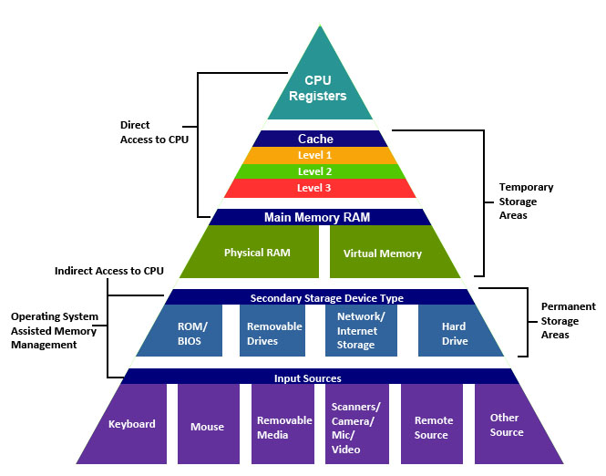
At the highest level of memory hierarchy, closest to the CPU, we have the CPU register. A processor register is a quickly accessible location available to a computer’s CPU. Registers usually consist of a small amount of fast storage and may be read-only or write-only. The CPU has super fast access to data stored in register. But the problem is that this memory is very small, typically on the orders of bits of information.

At the second level of the hierarchy of memory, we have the CPU cache, typically comprised of three different levels L1, L2, L3, which rank from fastest to slowest respectively, in terms of CPU access. However, the faster the cache memory, the smaller it is. Therefore, L1 is the fastest of the three, but also the smallest of the three levels.

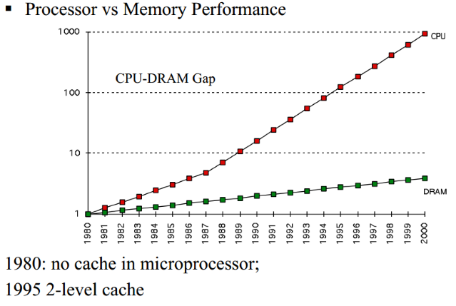
CPU Caching was invented to solve a significant problem. In the early decades of computing, main memory was extremely slow and incredibly expensive — but CPUs weren’t particularly fast, either. Starting in the 1980s, the gap began to widen quickly. Microprocessor clock speeds took off, but memory access times improved far less dramatically. As this gap grew, it became increasingly clear that a new type of fast memory was needed to bridge the gap. See the figure below.

After CPU cache, there the Random Access Memory (RAM) which you hear the most about, when you go to buy a new computer. Typical computers contain 4-32 Gb of RAM. When you open MATLAB and create some variables, all of your data is stored on this memory. However, this memory is the slowest of all in terms of access to CPU.

When you use for-loops in MATLAB to perform some specific calculations on a vector, you are asking MATLAB to go to this memory at each loop iteration to fetch an element of the loop, bring it to the CPU, perform the set of operations requested, and send it back to memory. However, the CPU is much more capable than doing a single calculation at a time. Therefore, if you could somehow tell MATLAB to fetch a bulk of elements from your vector and bring them to CPU to perform the requested operations, your code would become much faster. The way to tell MATLAB to do so, is called vectorization. By vectorizing your code, you tell MATLAB to bring as much information as possible to the highest memory level close to CPU, in order to perform the operations on all of them simultaneously and return the result for all of them back to the memory all together. This results in much faster code, since nowadays, as the figure above shows, the bottleneck in code performance is not the CPU speed, but the memory access.

Measuring the performance of your MATLAB functions and scripts

MATLAB has several built-in methods of timing how long it takes to run a MATLAB function or script. The timeit() function as well as tic and toc, are in particular very useful. Use the timeit() function for a rigorous measurement of your function’s execution time. Use tic and toc to estimate time for smaller portions of code that are not complete functions.

For additional details about the performance of your code, such as function call information and execution time of individual lines of code, MATLAB has more sophisticated tools such as MATLAB® Profiler.

Timing MATLAB functions

To measure the time required to run a function, whether built-in or your own, you can use the timeit() function. The timeit() function calls the user-specified function multiple times, and returns the median of the time measurements. This function takes a handle to the function whose performance is to be measured and returns the typical execution time, in seconds.

For example, suppose that you want to measure the performance of MATLAB’s built-in function, isprime() for a given input value to this function. You can compute the time to execute the function using timeit() like the following,

>> timeit( @()isprime(10^14) ) % pass the function as a handle to timeit()
ans =
    0.0787

Note that, this function isprime() will have different performance given different input numbers,

>> timeit( @()isprime(10^4) ) % pass the function as a handle to timeit()
ans =
   2.0402e-05

Time Portions of Code

To estimate how long a portion of your program takes to run or to compare the speed of different implementations of portions of your program, you can use MATLAB stopwatch timer functions: tic and toc. Invoking tic starts the timer, and the next toc reads the elapsed time.

tic
   % The program section to time. 
toc

Sometimes programs run too fast for tic and toc to provide useful data. If your code is faster than 1/10 second, consider timing it while running in a loop, and then average the result to find the time for a single run of the loop.

The cputime() function vs. tic/toc and timeit()

There is another MATLAB function that can do timing of your scripts or your functions: The cputime() function measures the total CPU time and sums across all threads (cores) in the CPU. This measurement is different from the wall-clock time that timeit() or tic/toc return, and could be misleading. For example, the CPU time for the pause function is typically small, but the wall-clock time accounts for the actual time that MATLAB execution is paused. Therefore, the wall-clock time might be longer.

If your function uses four processing cores equally, the CPU time could be approximately four times higher than the wall-clock time.

Frequently, your best choice to measure the performance of your code is timeit() or tic and toc. These functions return wall-clock time. Note that, unlike tic and toc, the timeit() function calls your code multiple times, and, therefore, considers the cost of first-time calls to your functions, which are typically more time-consuming than subsequent calls.

Some tips for Measuring Performance

• Always time a significant enough portion of code. Normally, the code that you are timing should take more than 1/10 second to run, otherwise the timing may not be very accurate.
  
  
• Put the code you are trying to time into a function instead of timing it at the command line or inside a script.
  
  
• Unless you are trying to measure first-time cost of running your code, run your code multiple times. Use the timeit() function for multiple calls timing of your function.
  
  
• Avoid clear all when measuring performance of your MATLAB scripts. This will add additional time to wipe MATLAB workspace from all current existing variable definitions, and therefore contaminate the timing measurements of the actual code in your MATLAB scripts.
  
  
• When performing timing measurements, assign your output to a variable instead of letting it default to ans().