This lecture discusses topics on data Input/Output processes in MATLAB.
Lecture Videos
This video is created solely as a reference for the attendants of ICP2017F course at UT Austin. If you did not attend this class, then you may not find this video useful.
So far in this course, we have indirectly discussed several methods of getting input information from the user, and several methods of outputting the result in a MATLAB program. This lecture, attempts at formalizing all the previous discussions and introduce more general efficient methods of code interaction with users.
Methods of data input/output in MATLAB
Let’s begin with an example code, explaining the meaning of input/output (I/O) in MATLAB,
a = 0.1;
b = 1;
x = 0.6;
y = a*exp(b*x)
0.1822
In the above code, a, b, x are examples of input data to a code, and y is an example of code output. In such cases as in the above, the input data is said to be hardcoded in the program.
NOTE
In general, in any programming language, including MATLAB, you should avoid hardcoding input information to your program as much as possible.
If data is hardcoded, then every time that it needs to be changed, the user has to change the content of the code. This is not considered good programming style for software development.
In general, input data can be fed to a program in four different ways:
- let the user answer questions in a dialog in MATLAB terminal window,
- let the user provide input on the operating system command line,
- let the user write input data in a graphical interface,
- let the user provide input data in a file.
For outputting data, there are two major methods,
- writing to the terminal window, as previously done using print() function, or,
- writing to an output file.
We have already extensively discussed printing output to the terminal window. Reading from and writing data to file is also easy as we see in this lecture.
Input/output from MATLAB terminal window
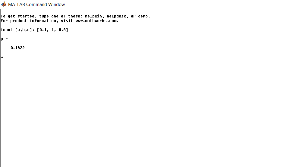
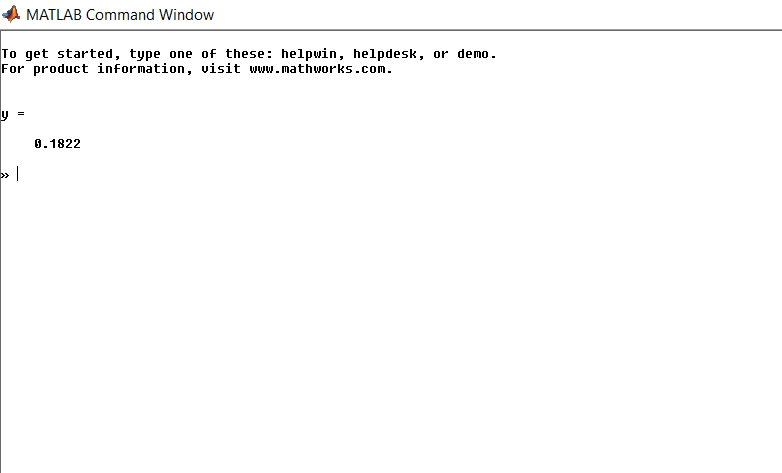
We have already introduced and used this method frequently in previous lectures, via the MATLAB’s built-in function input(). If we were to get the input data for the above code via the terminal window, an example approach would be the following,
datain = input('input [a,b,c]: ');
a = datain(1);
b = datain(2);
x = datain(3);
y = a*exp(b*x)
input a,b,c: [0.1, 1, 0.6]
y =
    0.1822
One could also read the input values as string ans then convert them to real values or parse the input using one of MATLAB’s built-in functions, for example,
>> datain = input('input [a,b,c]: ','s');
input [a,b,c]: [0.1, 1, 0.6]
>> class(datain)
ans =
char
>> datain = str2num(datain)
datain =
    0.1000    1.0000    0.6000
>> class(datain)
ans =
double
>> a = datain(1);
>> b = datain(2);
>> x = datain(3);
>> y = a*exp(b*x)
y =
    0.1822
Input/output data from operating system’s command line
This approach is most popular in Unix-like environments, where most users are accustomed to using Bash command line. However, it can be readily used in Windows cmd environment as well. For this approach, we have to invoke MATLAB from the computer operating system’s command line, that is, Bash in Linux systems, and cmd in Windows,
start matlab -nosplash -nodesktop -r "testIO
Then a MATLAB command-line window opens in your computer like the following that runs automatically your code (stored in testIO.m).
In the above command, we are basically starting MATLAB from the OS command line with our own choice of optional arguments for MATLAB. You can specify startup options (also called command flags or command-line switches) that instruct the MATLAB program to perform certain operations when you start it. On all platforms, specify the options as arguments to the matlab command when you start at the operating system prompt. For example, the following starts MATLAB and suppresses the display of the splash screen (a splash screen is a graphical control element consisting of a window containing an image, a logo, and the current version of the software. A splash screen usually appears while a game or program is launching),
matlab -nosplash
The flag -nodesktop result in opening only the MATLAB command line, and no MATLAB Graphical user interface (GUI) just like the figure above. Finally, the flag -r executes the MATLAB file that appears right after it, specified as a string or as the name of a MATLAB script or function. If statement is MATLAB code, you should enclose the string with double quotation marks. If statement is the name of a MATLAB function or script, do not specify the file extension and do not use quotation marks. Any required file must be on the MATLAB search path or in the startup folder. You can also set MATLAB’s working folder right from the command-line using -sd flag. You can find find more information about all possible flags here. On Windows platforms, you can precede a startup option with either a hyphen (-) or a slash (/). For example, -nosplash and /nosplash are equivalent.
Note that you can also quote MATLAB on the OS command line, along with the name of the script you want to run. For example, suppose you wanted to run the original script,
a = 0.1;
b = 1;
x = 0.6;
y = a*exp(b*x)
but now with a, b, x, given at runtime. You could write a script file test.m that contains,
y = a*exp(b*x)
and give the variables values at runtime, on OS command line, like the following,
matlab -nosplash -nodesktop -r "a = 0.1; b = 1; x = 0.6; testIO"
The figure below shows a screen-shot illustrarting the output of the above command.
Input/output data from a Graphical User Interface
This method of inputting data is done by constructing a Graphical User Interface (GUI) which opens and takes input from the user. This is probably one of the most convenient methods for the users to input data. You can do this in MATLAB for example by using the built-in function inputdlg() which creates dialog box that gathers user input. But this method of data colleciton is beyond the scope of our class. More information about this can be found here.
Input/output data from file
In cases where the input/output data is large, the command-line arguments and input from terminal window are not efficient anymore. In such cases, the most common approach is to let the code read/write data from a pre-existing file, the path to which is most often given to the code via the OS command line or MATLAB terminal window.
There are many methods of importing and exporting data to and from MATLAB, only some of which we will discuss here. For more information see here, here, and here. The following table shows some of the most important import functions in MATLAB, which we will discuss here as well.
| Function | Description |
|---|---|
load() | Load MATLAB variables from file into MATLAB workspace |
save() | save MATLAB variables from MATLAB workspace into a MATLAB `.mat` file. |
fscanf() | Read data from text file |
fprintf() | Write data to a text file |
dlmread() | Read ASCII-delimited file of numeric data into matrix |
dlmwrite() | Write a numeric matrix into ASCII-delimited file |
csvread() | Read comma-separated value (CSV) file |
csvwrite() | Write values of a matrix into a comma-separated (CSV) file |
xlswrite() | Read Microsoft Excel spreadsheet file |
xlswrite() | write data into a Microsoft Excel spreadsheet file |
readtable() | Create table from file |
writetable() | Write table to file |
imread() | Read image from graphics file |
imwrite() | Write image to graphics file |
importdata() | Load data from file |
textscan() | Read formatted data from text file or string |
fgetl() | Read line from file, removing newline characters |
fread() | Read data from binary file |
fwrite() | Write data to binary file |
type() | Display contents of file |
Loading/saving MATLAB workspace variables
MATLAB has two useful functions that can save the workspace variables into special MATLAB .mat files, to be later load again into the same or another MATLAB workspace for further work or manipulation. The function save() saves workspace variables to a given file. The most useful options for this function are the following,
save(filename)
save(filename,variables)
save(filename,variables,fmt)
save(filename)saves all variables from the current workspace in a MATLAB formatted binary file called MAT-file with the given namefilename. If the filefilenameexists,save()overwrites the file.
save(filename,variables)saves only the variables or fields of a structure array specified byvariables. For example,p = rand(1,10); q = ones(10); save('pqfile.mat','p','q')
will create the binary MAT file pqfile.mat which contains the two variables.
save(filename,variables,fmt)saves the requested variables with the file format specified byfmt. The variables argument is optional. If you do not specify variables, the save function saves all variables in the workspace. File format, specified as one of the following. When using the command form of save, you do not need to enclose the input in single or double quotes, for example, save myFile.txt -ascii -tabs.
| Value of fmt | File Format |
|---|---|
'-mat' | Binary MAT-file format. |
'-ascii' | Text format with 8 digits of precision. |
'-ascii','-tabs' | Tab-delimited text format with 8 digits of precision. |
'-ascii','-double' | Text format with 16 digits of precision. |
'-ascii','-double','-tabs' | Tab-delimited text format with 16 digits of precision. |
For example,
p = rand(1,10);
q = ones(10);
save('pqfile.txt','p','q','-ascii')
will create an ASCII text file pqfile.txt which contains the two variables p and q.
Similarly, one can reload the same files into MATLAB workspace again if needed, for example using MATLAB load() function,
>> load('pqfile.txt')
>> pqfile
pqfile =
  Columns 1 through 8
    0.0975    0.2785    0.5469    0.9575    0.9649    0.1576    0.9706    0.9572
    1.0000    1.0000    1.0000    1.0000    1.0000    1.0000    1.0000    1.0000
    1.0000    1.0000    1.0000    1.0000    1.0000    1.0000    1.0000    1.0000
    1.0000    1.0000    1.0000    1.0000    1.0000    1.0000    1.0000    1.0000
    1.0000    1.0000    1.0000    1.0000    1.0000    1.0000    1.0000    1.0000
    1.0000    1.0000    1.0000    1.0000    1.0000    1.0000    1.0000    1.0000
    1.0000    1.0000    1.0000    1.0000    1.0000    1.0000    1.0000    1.0000
    1.0000    1.0000    1.0000    1.0000    1.0000    1.0000    1.0000    1.0000
    1.0000    1.0000    1.0000    1.0000    1.0000    1.0000    1.0000    1.0000
    1.0000    1.0000    1.0000    1.0000    1.0000    1.0000    1.0000    1.0000
    1.0000    1.0000    1.0000    1.0000    1.0000    1.0000    1.0000    1.0000
  Columns 9 through 10
    0.4854    0.8003
    1.0000    1.0000
    1.0000    1.0000
    1.0000    1.0000
    1.0000    1.0000
    1.0000    1.0000
    1.0000    1.0000
    1.0000    1.0000
    1.0000    1.0000
    1.0000    1.0000
    1.0000    1.0000
But note that upon loading the Ascii file, the information about the individual variables is lost. By contrast, loading data using the MAT file will preserve the variables structure,
>> load('pqfile.mat')
>> p
p =
  Columns 1 through 8
    0.1419    0.4218    0.9157    0.7922    0.9595    0.6557    0.0357    0.8491
  Columns 9 through 10
    0.9340    0.6787
>> q
q =
     1     1     1     1     1     1     1     1     1     1
     1     1     1     1     1     1     1     1     1     1
     1     1     1     1     1     1     1     1     1     1
     1     1     1     1     1     1     1     1     1     1
     1     1     1     1     1     1     1     1     1     1
     1     1     1     1     1     1     1     1     1     1
     1     1     1     1     1     1     1     1     1     1
     1     1     1     1     1     1     1     1     1     1
     1     1     1     1     1     1     1     1     1     1
     1     1     1     1     1     1     1     1     1     1
Reading/writing a formatted file using fscanf() and fprintf()
There are numerous methods of reading the contents of a file in MATLAB. The most trivial and probably least pleasing method is through MATLAB’s built-in function fscanf(). To read a file, say this file, you will have to first open it in MATLAB,
fileID = fopen('data.in','r');
formatSpec = '%f';
A = fscanf(fileID,formatSpec)
fclose(fileID);
A =
    1
    3
    4
    5
    6
    7
    88
    65
Note that unlike the C language’s fscanf(), in MATLAB fscanf() is vectorized meaning that it can read multiple lines all at once. Here, the attribute 'r' states that the file is opened for the purpose of reading it (vs writing, or some other purpose). A list of available options for fopen() are the following,
| Attribute | Description |
|---|---|
'r' | Open file for reading. |
'w' | Open or create new file for writing. Discard existing contents, if any. |
'a' | Open or create new file for writing. Append data to the end of the file. |
'r+' | Open file for reading and writing. |
'w+' | Open or create new file for reading and writing. Discard existing contents, if any. |
'a+' | Open or create new file for reading and writing. Append data to the end of the file. |
'A' | Open file for appending without automatic flushing of the current output buffer. |
'W' | Open file for writing without automatic flushing of the current output buffer. |
The general syntax for reading an array from an input file using fscanf() is the following,
array = fscanf(fid,format)
[array, count] = fscanf(fid,format,size)
where the optional argument size specifies the amount of data to be read from the file. There are three versions of this argument,
n: Reads exactlynvalues. After this statement,arraywill be a column vector containingnvalues read from the file.Inf: Reads until the end of the file. After this statement,arraywill be a column vector containing all of the data until the end of the file.[n m]: Reads exactly, $n\times m$ values, and format the data as an $n\times m$ array. For example, consider this file, which contains two columns of numeric data. One could read this data usingfscanf()like the following,>> formatSpec = '%d %f'; >> sizeA = [2 Inf]; >> fileID = fopen('nums2.txt','r'); >> A = transpose(fscanf(fileID,formatSpec,sizeA)) >> fclose(fileID); A = 1.0000 2.0000 3.0000 4.0000 5.0000 0.8147 0.9058 0.1270 0.9134 0.6324
Now suppose you perform some on operation onA, say the elemental multiplication ofAby itself. Then you want to store (append) the result into another file. You can do this using MATLAB functionfprintf(),>> formatSpec = '%d %f \n'; >> fileID = fopen('nums3.txt','w+'); >> fprintf(fileID,formatSpec,A.*A); >> fclose(fileID);
The optionw+tells MATLAB to store the result in a file named num3.txt, and if the file does already exist, then append the result to the end of the current existing file. To see what formatting specifiers you can use with MATLABfscanf()andfprintf(), see this page.
MATLAB also has some rules to skip characters that are unwanted in the text file. These rules are really details that are specific to your needs and the best approach is to seek the solution to your specific problem by searching MATLAB’s manual or the web. For example, consider this file which contains a set of temperature values in degrees (including the Celsius degrees symbol). One way to read this file and skipping the degrees symbol in MATLAB could be then the following set of commands,
>> fileID = fopen('temperature.dat','r');
>> degrees = char(176);
>> [A,count] = fscanf(fileID, ['%d' degrees 'C'])
>> fclose(fileID);
A =
    78
    72
    64
    66
    49
count =
     5
This method of reading a file is very powerful but rather detailed, low-level and cumbersome, specially that you have to define the format for the content of the file appropriately. Most often, other higher-level MATLAB’s built-in function come to rescue us from the hassles of using fscanf(). For more information about this function though, if you really want to stick to it, see here. Some important MATLAB special characters (escape characters) that can also appear in fprintf() are also given in the following table.
| Symbol | Effect on Text |
|---|---|
'' | Single quotation mark |
%% | Single percent sign |
\\ | Single backslash |
\n | New line |
\t | Horizontal tab |
\v | Vertical tab |
Reading/writing data using dlmread()/dlmwrite() and csvread()/csvwrite()
The methods discussed above are rather primitive, in that they require a bit of effort by the user to know something about the structure of the file and its format. MATLAB has a long list of advanced IO functions that can handle a wide variety of data file formats. Two of the most common functions are dedicated specifically to read data files containing delimited data sets: csvread() and dlmread().
In the field of scientific computing, a Comma-Separated Values (CSV) data file is a type of file with extension .csv, which stores tabular data (numbers and text) in plain text format. Each line of the file is called a data record and each record consists of one or more fields, separated by commas. The use of the comma as a field separator is the source of the name for this file format.
Now suppose you wanted to read two matrices whose elements were stored in CSV format in two csv data files matrix1.csv and matrix2.csv. You can accomplish this task simply by calling MATLAB’s built-in csv-reader function called csvread(filename). Here the word filename is the path to the file in your local hard drive. For example, download these two given csv files above in your MATLAB working directory and then try,
>> Mat1 = csvread('matrix1.csv');
>> Mat2 = csvread('matrix2.csv');
Then suppose you want to multiply these two vectors and store the result in a new variable and write it to new output csv file. You could do,
Mat3 = Mat1 * Mat2;
>> csvwrite('matrix3.csv',Mat3)
which would output this file: matrix3.csv for you.
Alternatively, you could also use MATLAB’s built-in functions dlmread() and dlmwrite() functions to do the same things as above. These two functions read and write ASCII-delimited file of numeric data. For example,
>> Mat1 = dlmread('matrix1.csv');
>> Mat2 = dlmread('matrix2.csv');
>> Mat3 = Mat1 * Mat2;
>> dlmwrite('matrix3.dat',Mat3);
Note that, dlmread() and dlmwrite() come with an optional argument delimiter of the following format,
>> dlmread(filename,delimiter)
>> dlmwrite(filename,matrixObject,delimiter)
where the argument delimiter is the field delimiter character, specified as a character vector or string. For, example in the above case, the delimiter is comma ','. In other cases, you could for example use white space ' ', or '\t' to specify a tab delimiter, and so on. For example, you could have equally written,
>> dlmwrite('matrix4.dat',Mat3,'\t');
to create a tab-delimited file named matrix4.dat.
Reading/writing data using xlsread() and xlswrite()
Once data becomes more complex than simple numeric matrices or vectors, then we need more complex MATLAB functions for IO. An example of such case, is when you have stored your information in Microsoft Excel file. For such cases, you can use xlsread(filename) to read the file specified by the input argument filename to this function. We will later on see some example usages of this function in homework. Similarly, you could write data into an excel file using xlswrite(). For example,
>> values = {1, 2, 3 ; 4, 5, 'x' ; 7, 8, 9};
>> headers = {'First','Second','Third'};
>> xlswrite('XlsExample.xlsx',[headers; values]);
would create this Microsoft Excel file for you.
Reading/writing data using readtable() and writetable()
Another important and highly useful set of MATLAB functions for IO are readtable() and writetable(). The function readtable() is used to read data into MATLAB in the form of a MATLAB table data type. For example, you could read the same Excel file that we created above into MATLAB using readtable() instead of xlsread(),
>> XlsTable = readtable('XlsExample.xlsx')
XlsTable =
    First    Second    Third
    _____    ______    _____

    1        2         '3'
    4        5         'x'
    7        8         '9'
Reading and writing image files using imread() and imwrite()
MATLAB has a really wide range of input/output methods of data. We have already discussed some of the most useful IO approaches in the previous sections. For graphics files however, none of the previous functions are useful. Suppose you wanted to import a jpg or png or some other type graphics file into MATLAB in order to further process it. For this purpose MATLAB has the built-in function imread() which can read image from an input graphics file. For example, to read this image file in MATLAB, you could do,
>> homer = imread('homer.jpg');
>> imshow(homer)
to get the following figure in MATLAB,

Now suppose you want to convert this figure to black-and-white and save it as a new figure. You could do,
>> homerBW = rgb2gray(homer);
>> imshow(homerBW)
>> imwrite(homerBW,'homerBW.png');
to get this black and white version of the above image, now in png format (or in any format you may wish, that is also supported by MATLAB).
Reading a file using importdata()
Probably, the most general MATLAB function for data input is importdata(). This function can be used to import almost any type of data and MATLAB is capable of automatically recognizing the correct format for reading the file, based on its extension and content. For example, you could read the same image file above, using importdata(),
>> newHomer = importdata('homer.jpg');
>> imshow(newHomer)
to import it to MATLAB. At the same time, you could also use it to import data from the excel file that we created above, XlsExample.xlsx,
>> newXls = importdata('XlsExample.xlsx')
newXls =
          data: [3x3 double]
      textdata: {3x3 cell}
    colheaders: {'First'  'Second'  'Third'}
or similarly, read a csv-delimited file like matrix3.csv,
>> newMat3 = importdata('matrix3.csv')
newMat3 =
  Columns 1 through 7
       62774      103230       77362       87168       65546       64837      100700
      104090      143080      104700      116500      108250      105400      111110
       80351      112850       89506      113890      106030       70235      110620
       99522      134130       73169      134190      117710       92878       94532
       59531      102750       91679      111350       80539       84693       96078
       58504       76982       52076       91449       80797       69246       61569
       76170      104310       93950      114860       89779      101530       87014
       91610      118380       90636      107840       91120       90247       84871
       85943      110670       73451      114410      100840      111660       77908
       82570       94427       57213       81175       79305       78718       68662
  Columns 8 through 10
       79446       78102      106570
      102950      116850      137810
      113210      108800      128700
       93013      119130      132700
       95750      100980      100450
       67044       80635       78006
       86355      103760      119710
       92649       98589      132660
       73117      109270       99401
       65283       66888      114030
In general, you can use importdata() to read MATLAB binary files (MAT-files), ASCII files and Spreadsheets, as well as images and audio files.
Reading a file using fgetl()
Another useful MATLAB function for reading the content of a file is fgetl() which can read a file line by line, removing the new line characters \n from the end of each line. The entire line is read as a string. For example, consider this file. One could read the content of this text file using the function fgetl() like the following,
>> fid = fopen('text.txt');
>> line = fgetl(fid)  % read line excluding newline character
line =
The main benefit of using a weakly-typed language is the ability to do rapid prototyping. The number of lines of code required to declare and use a dynamically allocated array in C (and properly clean up after its use) are much greater than the number of lines required for the same process in MATLAB.
>> line = fgetl(fid)  % read line excluding newline character
line =
     ''
>> line = fgetl(fid)  % read line excluding newline character
line =
Weak typing is also good for code-reuse. You can code a scalar algorithm in MATLAB and with relatively little effort modify it to work on arrays as well as scalars. The fact that MATLAB is a scripted instead of a compiled language also contributes to rapid prototyping.
>> fclose(fid);
Reading data from web using webread()
In today’s world, it often happens that the data you need for your research is already stored somewhere on the world-wide-web. For such cases MATLAB has built-in methods and functions to read and import data or even a webpage. For example, consider this page on this course’s website. It is indeed a text file containing a set of IDs for some astrophysical events. Suppose, you needed to read and store these IDs locally on your own device. You could simply try the following code in MATLAB to fetch all of the table’s information in a single string via,
>> webContent = webread('https://www.cdslab.org/ICP2017F/homework/5-problems/triggers.txt')
webContent =
    '00745966
     00745090
     00745022
     00744791
     00741528
     00741220
     00739517
     00737438
     ...
     00100319'
>>
Now if we wanted to get the individual IDs, we could simply use strplit() function to split the IDs at the line break characters '\n',
>> webContent = strsplit(webContent,'\n')
webContent =
  1×10¹⁹ cell array
  Columns 1 through 11
    {'00745966'}    {'00745090'}    {'00745022'} ...
We will see more sophisticated usages of this MATLAB function in the first problem of homework 5.
Handling IO errors
A good code has to be able to handle exceptional situations that may occur during the code execution. These exceptions may occur during data input from either command line, terminal window, or an input file. They may also occur as a result of repeated operations on the input data, inside the code. For example, in previous homework assignments, we have learned some simple ways of handling the wrong number of input arguments, for example in Fibonacci sequence problem. This and similar measures to handle nicely the unexpected runtime errors are collectively called error and exception handling.
A simple way of error handling is to write multiple if-blocks, each of which handles a special exceptional situation. That is, to let the code execute some statements, and if something goes wrong, write the program in such a way that can detect this and jump to a set of statements that handle the erroneous situation as desired.
A more modern and flexible way of handling such potential errors in MATLAB is through MATLAB’s try/catch construction. You can use a try/catch statement to execute code after your program encounters an error. try/catch statements can be useful when you Want to finish the program in another way that avoids errors (which could lead to abrupt interruption of the program), or when you want to nicely control the effects of error (for example, when a division by zero happens in your calculations), or you have a function that could take many problematic parameters or commands as input, just like the fib function we wrote in the previous homework assignments.
The general syntax for try/catch statements is like the following pseudocode,
try
  try statements (all the normal things you would want to do)...
catch exception
  catch block (things to do when the try statements go wrong) ...
end
If an error occurs within the try block, MATLAB skips any remaining commands in the try block and executes the commands in the catch block. If no error occurs within try block, MATLAB skips the entire catch block.
For example, suppose we wanted to read data from a webpage that does not exist,
>> webContent = webread('https://www.cdslab.org/ICP2017F/homework/5-problems/')
Error using readContentFromWebService (line 45)
The server returned the status 404 with message "Not Found" in response to the request to URL https://www.cdslab.org/ICP2017F/homework/5-problems/.
Error in webread (line 125)
[varargout{1:nargout}] = readContentFromWebService(connection, options);
In such cases, it would be nice to control the behavior of the problem, and not allow MATLAB to end the program abruptly. We could therefore say,
>> try
    webContent = webread('https://www.cdslab.org/ICP2017F/homework/5-problems/')
catch
    disp('The requested page does not exist! Gracefully exiting...')
end
The requested page does not exist! Gracefully exiting...
Now, the true advantage of this error handling construct would become clear to you when you use it in functions. We will see more of this in homework 5.