This lecture aims at teaching you the how to of programming, difference between programming languages and the natural languages, the type of programming errors and the meaning code debugging how to perform simple arithmetic operations on the MATLAB command line.

For general information on MATLAB Data Types, see MATLAB manual.

Lecture Videos

This video is created solely as reference for the attendants of ICP2017F course at UT Austin. If you did not attend this class, then you may not find this video useful. For this lecture, video 4.0 was currupt, and could not be uploaded here.

Programming glossary

The following table contains some technical programming phrases that are often used and heard in the field of computer science and programming, that you need to be familiar as well.

Table 1. Some programming phrases that are discussed in this lecture. The boldface words in the description column indicate items that are expressions with their own description in this table.

Expression	Description
algorithm	A general method for solving a class of problems.
bug	An error in program that has to be resolved for successful execution of the program.
compiled language	A programming language whose programs need to be compiled by a compiler in order to run.
compiler	A software that translates an entire high-level program into a lower-level language to make it executable.
debugging	The process of finding and removing any type of error in the program.
exception	An alternative name for runtime error in the program.
executable	An object code, ready to be executed. Generally has the file extension .exe or .out or no extension at all.
formal language	A language that is intentionally designed for specific purposes, which, unlike natural languages, follows a strict standard.
high-level language	A programming language (e.g., MATLAB, Python, Fortran, Java, etc) that has high level of abstraction from the underlying hardware.
interpreted language	A programming language whose statements are interpreted line-by-line by an interpreter and immediately executed.
low-level language	A programming language that has a low-level of abstraction from computer hardware and architecture, such as Assembly. Very close to machine code.
natural language	A language that evolves naturally, and has looser syntax rules and standard compared to formal languages.
object code	The output of a compiler after translating a program.
parsing	Reading and examining a file/program and analyzing the syntactic structure of the file/program.
portability	A program's ability to be executable on more than one kind of computer architecture, without changing the code.
problem solving	The process of formulating a problem and finding and expressing a solution to it.
program	A set of instructions in a that together specify an algorithm a computation.
runtime error	An error that does not arise and cause the program to stop, until the program has started to execute.
script	A program in an interpreted language stored in a file.
semantic error	A type of error in a program that makes the program do something other than what was intended. Catching these errors can be very tricky.
semantics	The meaning of a program.
source code	A program in a high-level compiled language, before being compiled by the compiler.
syntax error	A type of error in program that violates the standard syntax of the programming language, and hence, the program cannot be interpreted or compiled until the syntax error is resolved.
syntax	The structure of a program.
token	One of the basic elements of the syntactic structure of a program, in analogy with word in a natural language.

The content of a computer program

Although different programming languages look different in their syntax standards, virtually all programming languages are comprised of the following major components (instructions):

1. input
   Virtually every program starts with some input data by the user, or the input data that is hard-coded in the program.
   
   
2. mathematical/logical operations
   Virtually all programs involve some sort of mathematical or logical operations on the input data to the program.
   
   
3. conditional execution
   In order to perform the above operations on data, most often (but not always) there is a need to chack if some conditions are met in the program, and then perform specific programming instructions corresponding to each of the conditions.
   
   
4. repetition / looping
   Frequently it is needed to perform a specific set of operations repeatedly in the program to achieve the program’s goal.
   
   
5. output
   At the end of the program, it is always needed to output the program result, either to computer screen, or to a file.

Debugging a program

As it is obvious from its name, a bug in a computer program is annoying programming error that needs fixing in order for the program to become executable or to give out the correct answer. The process of removing program bugs is called debugging. There are basically three types of programming bugs (errors):

1. syntax error
   
   A program, weather interpreted or compiled, can be successfully run only if it is syntactically correct. Syntax errors are related to the structure and standard of the language, and the order by which the language tokens are allowed to appear in the code. For example, when you write your first MATLAB Hello World script, you would write,

   >> disp('Hello World!')
   Hello World!
   

   
   or,

   >> disp 'Hello World!';
   Hello World!
   

   
   However, if you type a wrong statement, MATLAB will give you a syntax error, like the following,

   >> disp(*Hello World!*)
    disp(*Hello World!*)
      ↑
   Error: Unexpected MATLAB operator.
   

   
   

2. runtime error
   
   Runtime errors or sometimes also named exceptions are a class of programming errors that can be detected only at the time of running the code, that is, they are not syntax errors. Examples include:
   
   
   • memory leaks (very common error in beginner C and C++ codes)
   • uninitialized memory
   • access request to illegal memory address of the computer
   • security attack vulnerabilities
   • buffer overflow
     These errors can be sometimes tricky to identify.
     
     
3. semantic error
   Unlike syntax errors that comprise of something the compiler/interpreter does not understand, semantic errors do not cause any compiler/interpreter error messages. However, the resulting compiled/interpreted code will NOT do what it is intended to do. Semantic errors are the most dangerous types of programming errors, as they do not raise any error flag by the compiler/interpreter, yet the program will not do what it is intended to do, although the code may look perfectly fine on its face. Semantic error is almost synonymous with logical error. Dividing two integers using the regular division operator / in MATLAB while expecting the result to be integer, would be a semantic error. This is because in MATLAB (unlike Fortran, for example), the regular division operator always outputs the result as real (float).

>> 2/7

ans =

    0.2857

>> class(ans)

ans =

double

Methods of running a MATLAB program

1. Writing MATLAB script on the MATLAB interpreter’s command prompt:
   Now, as you may have noticed, in the above example, I used MATLAB command line to code my first simple MATLAB script. This is one of the simplest and quickest method of MATLAB scripting and is actually very useful for testing small simple MATLAB ideas and code snippets on-the-fly.
   
   
2. Running MATLAB code written in a MATLAB .m file from MATLAB command prompt:
   As the program size grows, it wiser to put all of your MATLAB script into a single .m file, and then let the MATLAB interpreter run (i.e., interpret) your entire file all at once. To save the above simple “Hello World” MATLAB code in a file and run it, open a new m-file in MATLAB editor, then paste the code in the file and save it in MATLAB’s current working directory as hello.m. Then you can either call your program on the command line as the following,
   

   >> hello
   Hello World!
   

   
   or, simply press F5 button on your keyboard to run it.

3. Running your MATLAB script file from the Bash/cmd command line: You can also run your codes directly from the Windows cmd or Linux Bash command lines by simply calling MATLAB, followed by a list of optional flags, followed by the name and path to your MATLAB script. For example,

   matlab -nodisplay -nodesktop -r "run /home/amir/matlab/hello.m"
   

   
   

4. Running MATLAB code as an standalone application by compiling it: You can also compile your MATLAB script into a binary file (machine language), which is then standalone and executable independently of MATLAB. This is however out of the scope of our course, but you can read more about it here.

MATLAB interpreter as a simple calculator

One of the greatest advantages of MATLAB is that it can be used as a simple calculator and program interpreter on-the-fly, just like Python, Mathematica, R, and other scripting languages. In the following, you will see why and how.

Values and their types in MATLAB

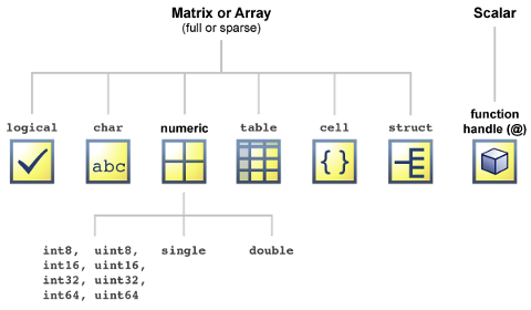
Values are one of the most fundamental entities in programming. Like any other language, a value in MATLAB can be of different types, most importantly Numeric (plain integer, long integer, float (real number), complex), Boolean (logical) which is a subtype of Numeric, or char (string), and many more. Each value type in MATLAB is a class. We will get to what classes are, at the end of the semester. For now, all you need to know is that there 6 main data types (in addition to function handles).

Numeric and logical values in MATLAB

The following are a few example arithmetic operations with values in MATLAB. You can perform very simple arithmetic on the MATLAB command line, and the result immediately by pressing enter.

>> 2 + 5 % Just typing some comment on the MATLAB command line. Anything after % is a comment and will be ignored.

ans =

     7

>> 2 - 7 % difference

ans =

    -5

>> 2 * 7 % product

ans =

    14

>> true % logical true value

ans =

     1

>> false % logical false value

ans =

     0

Obtaining the type (i.e. class) of a value

You can use the MATLAB’s built-in function class to get the type of a value in MATLAB (Of course, this is somewhat obvious and redundant for a value as we already readily know the type of a value).

>> class(2*7) % class function gives you the type of the input object to function "class"

ans =

double

>> class('This is a MATLAB string (char)') % a char value in MATLAB

ans =

char

>> class("This is a MATLAB string") % Note that you cannot use quotation marks for representing string values.
 class("This is a MATLAB string") % Note that you cannot use quotation marks for representing string values.
       ↑
Error: The input character is not valid in MATLAB statements or expressions.

>> class(1)

ans =

double

>> class(class(1))

ans =

char

>> class(true)

ans =

logical

>> class(false)

ans =

logical

vector and matrix values

Vectors and matrices are used to represent sets of values, all of which have the same type. A matrix can be visualized as a table of values. The dimensions of a matrix are $rows \times cols$, where $rows$ is the number of rows and $cols$ is the number of columns of the matrix. A vector in MATLAB is equivalent to a one-dimensional array or matrix.

Creating row-wise and column-wise vectors

Use , or space to separate the elements of a row-wise vector.

>> [1 2 3 4] % a space-separated row vector

ans =

     1     2     3     4

>> class([1 2 3 4])

ans =

double

>> [1, 2, 3, 4] % a comma-separated row vector

ans =

     1     2     3     4

>> class([1, 2, 3, 4])

ans =

double

Use ; to separate the elements of a column-wise vector.

>> [1; 2; 3; 4] % a column vector

ans =

     1
     2
     3
     4

>> class([1; 2; 3; 4])

ans =

double

Creating matrix values

Use ; to separate a row of matrix from the next.

>> [1,2,3,4;5,6,7,8;9,10,11,12] % a 3 by 4 matrix

ans =

     1     2     3     4
     5     6     7     8
     9    10    11    12

Cells and tables

Matrices and vectors can only store numbers in MATLAB. If one needs a more general array representation for a list of strings for example, then one has to use cells or tables.

Cell array values

Cell arrays, are array entities that can contain data of varying types and sizes. A cell array is a data type with indexed data containers called cells, where each cell can contain any type of data. Cell arrays commonly contain either lists of text strings, combinations of text and numbers, or numeric arrays of different sizes. Refer to sets of cells by enclosing indices in smooth parentheses, (). Access the contents of cells by indexing with curly braces, {}. Also, to define a cell, use {} like the following notation,

>> {'Hi', ' ', 'World!'} % a cell array of strings

ans = 

    'Hi'    ' '    'World!'

>> class({'Hi', ' ', 'World!'})

ans =

cell

>> {'Hi', 1, true, 'World!'}

ans = 

    'Hi'    [1]    [1]    'World!'

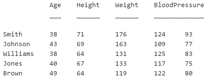
Table values

MATLAB tables are arrays in tabular form whose named columns can have different types. Table is a data type suitable for column-oriented or tabular data that is often stored as columns in a text file or in a spreadsheet. Tables consist of rows and column-oriented variables. Each variable in a table can have a different data type and a different size with the one restriction that each variable must have the same number of rows.

Later on, we learn more about Tables and Cells in MATLAB, once we introduce MATLAB variables.

Value coercion in MATLAB

Value coercion is the implicit process by which the MATLAB interpreter/compiler automatically converts a value of one type into a value of another type when that second type is required by the surrounding context. For example:

>> class(int32(1.0)) % int32 gives a 32-bit (4-byte) integer.
ans =

int32

>> int32(2.0) * int32(1.0) % Note that the product of two integers, is integer.

ans =

           2

>> class(ans)

ans =

int32

>> int32(1.0) * 2.5 % Note that the product of float and integer, is coerced into an integer!

ans =

           3

>> class(ans)

ans =

int32

>> int32(1.0) / 2.5 % Note that the division of float and integer, is coerced into an integer.

ans =

           0

>> 2.0 / 7 % floating point division with float result

ans =

    0.2857

>> true + 1 % logical and double are coerced into double

ans =

     2

>> class(true + 1)

ans =

double

But note that,

>> true + int32(1) % you cannot combine logical with integer
Error using  + 
Integers can only be combined with integers of the same class, or scalar doubles.

>> true + false

ans =

     1

>> true * false

ans =

     0

>> true / false
Undefined operator '/' for input arguments of type 'logical'.

ATTENTION

As you saw above, unlike other languages, such as Python, integer value has precedence over float, that is, the result of the calculation is coerced into an integer.

ATTENTION

I recommend you to always explicitly write the type of each value in your calculations or your MATLAB scripts. For example, denote all floats by adding a decimal point . to each float (real) value.

Some further useful MATLAB commands

MATLAB has a built-in function called format that can modify the output style of MATLAB on the command line. For example,

>> 2/5

ans =

    0.4000

>> format long
>> 2/5

ans =

   0.400000000000000

>> format short
>> 2/5

ans =

    0.4000

>> format compact
>> 2/5
ans =
    0.4000
>> format loose
>> 2/5

ans =

    0.4000

Here is a complete list of options that format can take,

Table 2. A list of MATLAB format options.

Style	Result	Example
short (default)	Short, fixed-decimal format with 4 digits after the decimal point.	3.1416
long	Long, fixed-decimal format with 15 digits after the decimal point for double values, and 7 digits after the decimal point for single values.	3.141592654
shortE	Short scientific notation with 4 digits after the decimal point.	3.14E+00
longE	Long scientific notation with 15 digits after the decimal point for double values, and 7 digits after the decimal point for single values.	3.14E+00
shortG	Short, fixed-decimal format or scientific notation, whichever is more compact, with a total of 5 digits.	3.1416
longG	Long, fixed-decimal format or scientific notation, whichever is more compact, with a total of 15 digits for double values, and 7 digits for singlevalues.	3.141592654
shortEng	Short engineering notation (exponent is a multiple of 3) with 4 digits after the decimal point.	3.14E+00
longEng	Long engineering notation (exponent is a multiple of 3) with 15 significant digits.	3.14E+00
+	Positive/Negative format with +, -, and blank characters displayed for positive, negative, and zero elements.	+
bank	Currency format with 2 digits after the decimal point.	3.14
hex	Hexadecimal representation of a binary double-precision number.	400921fb54442d18
rat	Ratio of small integers.	355/113