This lecture further explains the concept of functions and different of types of it in MATLAB.

Useful link: Comprehensive MATLAB function list

Lecture Videos

This video is created solely as reference for the attendants of ICP2017F course at UT Austin. If you did not attend this class, then you may not find this video useful.

Function handles in MATLAB

Function Handles are variables that allow you to invoke a function indirectly. A function handle is a data type that stores an association to a function. For example, you can use a function handle to construct anonymous functions or specify call-back functions. Also, you can use a function handle to pass a function to another function, or call local functions from outside the main function (see below).

Indirectly calling a function enables you to invoke the function regardless of where you call it from. Typical uses of function handles include:

• Pass a function to another function (often called function functions). For example, passing a function to integration or optimization functions as we will see later in this course, such as integral and fzero.
• Construct handles to functions defined inline instead of stored in a program file (anonymous functions).
• Call local functions from outside the main function.

You can see if a variable, say h, is a function handle using isa(h,'function_handle').

Creating function handle

The general method for creating a function handle is to precede the function name with an @ sign. For example, if you have a function called myfunc, you can create a handle named f for it as follows,

f = @myfunc;

For example,

function out = getSq(x)
    out = x.^2;
end

Then you can create a function handle on MATLAB command line like the following,

>> f = @getSq;
>> a = 4;
>> b = f(a)
b =
    16

If the function does not require any inputs, then you can call the function with empty parentheses. For example,

>> h = @ones;
>> a = h()
a =
     1

If you don’t add () at the time of call, then simply another function handle will be created, now assigned to a,

>> h = @ones;
>> a = h
a = 
    @ones
>> class(a)
ans =
function_handle

Function handles can be passed as variables to other functions. For example, to calculate the integral of $f(x)=x^2$, as implemented in getSq() above, on the range $[0,1]$ define,

>> f = @getSq; 
>> q = integral(f,0,1)
q =
    0.3333

Arrays of function handles

You can also create an array of function handles by collecting them into a cell or structure array. For example,

>> fset = {@sin, @cos, @tan, @cot};
>> fset{1}(pi)
ans =
   1.2246e-16
>> fset{2}(pi)
ans =
    -1
>> fset{3}(pi)
ans =
  -1.2246e-16
>> fset{4}(pi)
ans =
  -8.1656e+15

To get general information about a function handle on MATLAB command line, use,

>> functions(fset{4})
ans = 
    function: 'cot'
        type: 'simple'
        file: ''

Function types in MATLAB

There are several types of functions in MATLAB. These include:

• local functions,
• nested functions,
• private functions,
• function functions,
• anonymous functions
• ….

Anonymous functions

Anonymous functions allow you to create a MATLAB file without the need to put the function in a separate .m file dedicated to the function. This function is associated with a variable whose data type is function_handle. Anonymous functions can accept inputs and return outputs, just as standard functions do. However, they can contain only a single executable statement. The concept of anonymous function is similar to lambda functions in Python, if you are already familiar with this language. For example, consider the following handle to an anonymous function that finds the square of a number,

>> sq = @(x) x.^2;
>> sq(2)
ans =
     4
>> sq([2,3,4])
ans =
     4     9    16

Variables in the anonymous function expressions

Function handles can store not only an expression, but also variables that the expression requires for evaluation. For example, you can create a function handle to an anonymous function that requires coefficients a, b, and c.

>> a = 1.3;
>> b = .2;
>> c = 30;
>> parabola = @(x) a*x.^2 + b*x + c;

Since a, b, and c are available at the time you create parabola, the function handle includes those values. The values persist within the function handle even if you clear the variables:

>> clear a b c
>> x = 1;
>> y = parabola(x)
y =
   31.5000

But note that in order to supply different values for the coefficients, you must create a new (e.g., redefine the) function handle,

>> a = -3.9;
>> b = 52;
>> c = 0;
>> parabola = @(x) a*x.^2 + b*x + c;
>> x = 1;
>> y = parabola(x)
y =
   48.1000

Multiple (nested) anonymous functions

The expression in an anonymous function can include another anonymous function. This is useful for passing different parameters to a function that you are evaluating over a range of values. For example, suppose you want to solve the following equation for varying values of the variable c,

$$g(c) = \int^1_0 \big( x^2 + cx + 1 \big) \operatorname{d}x$$

You can do so by combining two anonymous functions,

g = @(c) (integral(@(x) (x.^2 + c*x + 1),0,1));

Here are the steps to derive the above nested anonymous function:

• Write the integrand as an anonymous function,

  @(x) (x.^2 + c*x + 1)
  

• Evaluate the function from zero to one by passing the function handle to integral,

  integral(@(x) (x.^2 + c*x + 1),0,1)
  

• Supply the value for c by constructing an anonymous function for the entire equation,

  g = @(c) (integral(@(x) (x.^2 + c*x + 1),0,1));
  

The final function allows you to solve the equation for any value of c. For example,

>> g(10)
ans =
    6.3333

Anonymous functions with no input

If your function does not require any inputs, use empty parentheses when you define and call the anonymous function. Otherwise, as stated above in function handles, you will simply create a new function handle. For example,

>> t = @() datestr(now);
>> d = t()
d =
23-May-2017 19:54:07

and omitting the parentheses in the assignment statement creates another function handle, and does not execute the function,

>> d = t
d = 
    @()datestr(now)

Anonymous functions with multiple inputs or outputs

Anonymous functions require that you explicitly specify the input arguments, as many as it may be, just the way you would for a standard function, separating multiple inputs with commas. For example, the following function accepts two inputs, x and y,

>> myfunc = @(x,y) (x^2 + y^2 + x*y);
>> x = 1;
>> y = 10;
>> z = myfunc(x,y)
z =
   111

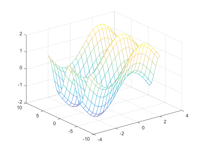
However, you do not explicitly define output arguments when you create an anonymous function. If the expression in the function returns multiple outputs, then you can request them when you call the function. In that case, you should enclose multiple output variables in square brackets []. For example, MATLAB’s ndgrid function can return as many outputs as the number of input vectors. This anonymous function that calls ndgrid can also return multiple outputs:

mygrid = @(x,y,c) ndgrid((-x:x/c:x),(-y:y/c:y));
[X,Y] = mygrid(pi,2*pi,10);

You can use the output from mygrid to create a mesh or surface plot, like the following, as we will further discuss in future lectures on plotting in MATLAB,

Z = sin(X) + cos(Y);
mesh(X,Y,Z)

Arrays of anonymous functions

As we did above for MATLAB function handles, you can also store multiple anonymous functions in a cell array or structure array. The most common approach is to use a cell array, like the following,

f = {@(x)x.^2;
     @(y)y+10;
     @(x,y)x.^2+y+10
     };

When you create the cell array, keep in mind that MATLAB interprets spaces as column separators for the cell array. Either omit spaces from expressions, as shown in the previous code, or enclose expressions in parentheses, such as

f = {@(x) (x.^2);
     @(y) (y + 10);
     @(x,y) (x.^2 + y + 10)
     };

Access the contents of a cell using curly braces. For example, f{1} returns the first function handle. To execute the function, pass input values in parentheses after the curly braces:

>> x = 1;
>> y = 10;
>> f{1}(x)
ans =
     1
>> f{2}(y)
ans =
    20
>> f{3}(x,y)
ans =
    21

Local functions

MATLAB program files can contain code for more than one function. In a function file, the first function in the file is called the main function. This function is visible to functions in other files, or you can call it from the command line. Additional functions within the file are called local functions, and they can occur in any order after the main function. Local functions are only visible to other functions in the same file. They are equivalent to subroutines in other programming languages, and are sometimes called subfunctions.

As of R2016b, you can also create local functions in a script file, as long as they all appear after the last line of script code. For more information, see here.

Exercise:
Create a function file named mystats.m that takes as input a given vector of real numbers, and outputs the mean and median of the vector. The .m file for this function should contain contains a main function mystats(), and two local functions, mymean and mymedian. Test your main function using an input vector like,

>> myvec = [10:3:100];
>> mystats(myvec)
ans =
    55

Collective function handle for all local functions

MATLAB has a built-in function localfunctions that returns a cell array of all local functions in the scope of the current function or script (i.e., in the current MATLAB file). This is very useful, when you want to write a function that returns to the main program, a list of functions local to this function. For example,

function fh = computeEllipseVals
    fh = localfunctions;
end

function f = computeFocus(a,b)
    f = sqrt(a^2-b^2);
end

function e = computeEccentricity(a,b)
    f = computeFocus(a,b);
    e = f/a;
end

function ae = computeArea(a,b)
    ae = pi*a*b;
end

Now, if you call computeEllipseVals on the command prompt, you will get a cell array to all functions local to computeEllipseVals,

>> fhcell = computeEllipseVals
ans = 
    @computeFocus       
    @computeEccentricity
    @computeArea
>> fhcell{3}(1,1) % get the area of an ellipse with semi-axes (1,1).
ans =
    3.1416

Function functions

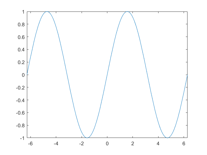
Function-functions are functions that operate on other functions that are passed to it as input arguments. The function that is passed to the function-function is usually referred to as passed function. A simple example is MATLAB’s built-in function fplot(func,lim), which plots the given input function func to it within the limit lim,

fplot(@sin,[-2*pi 2*pi])

Nested functions

Nested functions, as implicitly described by their names, are completely contained within a parent function. Any function in a program file can include a nested function. For example, consider the following simple function nestedfunc() inside of its parent function parent():

function parent
    disp('This is the parent function')
    nestedfunc
    function nestedfunc
       disp('This is the nested function')
    end
end

>> parent
This is the parent function
This is the nested function

The primary difference between nested functions and other types of functions is that they can access and modify variables that are defined in their parent functions. Therefore, nested functions can use variables that are not explicitly passed as input arguments. In a parent function, you can create a handle to a nested function that contains the data necessary to run the nested function.

Requirements for Nested Functions:

• Although MATLAB functions do not typically require an end statement, in order to nest any function in a program file, all functions in that file must use an end statement.
  
  
• You cannot define a nested function inside any of the MATLAB program control statements, such as if/elseif/else, switch/case, for, while, or try/catch.
  
  
• You must call a nested function either directly by name (without using feval), or using a function handle that you created using the @ operator (and not str2func).
  
  
• All of the variables in nested functions or the functions that contain them must be explicitly defined. That is, you cannot call a function or script that assigns values to variables unless those variables already exist in the function workspace.
  
  
• In general, variables in one function workspace are not available to other functions. However, nested functions can access and modify variables in the workspaces of the functions that contain them. This means that both a nested function and the parent function that contains it can modify the same variable without passing that variable as an argument. For example, in each of these functions, main1() and main2, both parent functions and the nested functions can access variable x,
  
  

  function main1
    x = 5;
    nestfun1
    function nestfun1 
        x = x + 1;
    end
    disp(['x = ',num2str(x)])
  end
  

  function main2
    nestfun2
    function nestfun2
        x = 5;
    end 
    x = x + 1;
    disp(['x = ',num2str(x)])
  end
  

  >> main1
  x = 5
  >> main1()
  x = 6
  >> main2()
  x = 6
  

  
  When the parent function does not use a given variable, the variable remains local to the nested function. This is rather subtle and complicated. So pay attention. For example, in this function named main, the two nested functions have their own versions of externFunc that cannot interact with each other, and calling main, gives a syntax error in nestedfun2, since myvar

  function main
    nestedfun1
    nestedfun2
    function nestedfun1
        myvar = 10;
        xyz = 5;
    end
    function nestedfun2
        myvar = myvar + 2;
    end
  end
  

  >> main
  Undefined function or variable 'myvar'.
  Error in main/nestedfun2 (line 10)
        myvar = myvar + 2;
  Error in main (line 3)
    nestedfun2
  

  
  However, even the slightest mention of the variable myvar, like the following, makes it accessible in the scope of both main and nested functions.

  function main
    nestedfun1
    nestedfun2
      
    function nestedfun1
        myvar = 10;
    end
  
    function nestedfun2
        myvar = myvar + 2;
    end
    disp(['myvar = ',num2str(myvar)]);
    disp(['class(myvar) = ',class(myvar)]);
  end
  

  >> main
  myvar = 12
  class(myvar) = double
  

  
  However, if there is any other function in MATLAB path that has the same name as this variable myvar, then MATLAB by default will call the function, instead of invoking the value for this variable given by the nested functions. For example if the following function is in MATLAB path,

  function result = myvar
    result = -13;
  end
  

  
  then calling the same function main as above would give,

  >> main
  myvar = -13
  class(myvar) = double
  

  
  The scope of variables in MATLAB functions, especially nested functions, can become a significant source of error and confusion in your MATLAB code, if you are not careful. As a result, MATLAB’s code editor, has special syntax-highlighting features for variables that are shared between nested functions, and is very smart in automatically detecting syntax or semantic errors in your codes. So, I always recommend you to use MATLAB’s own editor and debugger. You can find more information about this issue here.

Private Functions

A typical modern MATLAB contains thousands of M-files on the user’s path, all accessible just by typing the name of the M-file. While this ease of accessing M-files is an advantage, it can lead to clutter and clashes of names, not least due to the presence of “helper functions” that are used by other functions but not intended to be called directly by the user. Private functions provide an elegant way to avoid these problems. Any functions residing in a directory called private are visible only to functions in the parent directory. They can therefore have the same names as functions in other directories. When MATLAB looks for a function it searches subfunctions, then private functions (relative to the directory in which the function making the call is located), then the current directory and the path. Hence if a private function has the same name as a nonprivate function (even a built-in function), the private function will be found first.

Recursive functions

In programming, a recursive function is a function that calls itself. Recursion is needed frequently in programming, although there might be better, more efficient ways of implementing many of the simple explanatory recursion examples that you find in programming books. A prominent and sometimes more efficient alternative to recursive programming is iterative methods (e.g., loops and vectorization, which is the topic of the next lecture). Nontrivial examples that require recursive programming are abundant, but go beyond the scope of this course. Ask me in person and I will give you some examples from my own research.

To begin, let’s write a simple function that takes in one positive integer $n$, and calculates its factorial,

$$n! = n \times (n-1) \times \cdots \times 1 ~.$$

function result=getFactorial(x)
    if (x<=0)
        result=1;
    else
        result=x*getFactorial(x-1);
    end
end

>> getFactorial(3)
ans =
     6

Exercise:
Consider the MATLAB intrinsic function strtok, which returns the first token (word) in a given string (sentence). Now, write a recursive MATLAB function that reverses the input sentence given by the user like the following,

>> reverseSentence('MATLAB is a rather strange but very powerful programming language')

language programming powerful very but strange rather a is MATLAB 

Answer:

function reverseSentence(string)
    % reverseSentence recursively prints the words in a string in reverse order    
    getToken(string)
    function getToken(string)
        [word, rest] = strtok(string);
        if ~isempty(rest)
            getToken(rest);
        end
        fprintf([word,' '])
    end
    fprintf('\n')
end

MATLAB’s intrinsic functions

You may have already notices that functions are among the most useful concepts in programming. In fact, MATLAB owes its popularity to more 10000 built-in functions that contains, and the number is growing every year. That means we don’t need to write programs for more than 10000 important general tasks that we may need to do everyday, for example, integration, differentiation, various types of plotting, root finding and many more.

A comprehensive list of MATLAB’s built-in functions is available in MATLAB manual. I recommend you to bookmark this link on your personal computer, in order to get help from it whenever you need. As reminder, the following list contains some useful MATLAB functions, some of which we also discussed in the previous sections. Search for their cool functionalities in MATLAB manual!

• doc
• func2str
• str2func
• fplot
• feval
• fzero
• which
• edit
• type

Note that you can use the first one (doc) to view the information all the rest, even itself!

Scope of variables in MATLAB

Variable scope refers to the extent of the code in which a variable can be referenced, accessed or modified, without resulting in an access error. We have already discussed that variables inside functions are local to the functions and not visible to other functions in MATLAB. Variables defined inside a function are called local variables. They reside in the corresponding workspaces of the functions. The scope of local variables and dummy arguments is limited to the function (that is, to their workspace) in which they are defined. If the function contains nested functions, the code in the nested functions can access all variables defined in their parent function.

Occasionally it is convenient to create variables that exist in more than one workspace including, possibly, the main workspace. This can be done using the global statement. Variables stored in the MATLAB workspace (i.e., global memory) are called global variables.

Global vs local variables

Frequently, we need data (variable) protection (encapsulation) provided by local variables defined inside functions. In general, you should always do your best to avoid using global variables everywhere in your codes as much as possible. For small projects and problems, this may not be a significant issue. However, in large scale problems, the use of global variables can cause significant confusion, poor efficiency of your code, and even wrong results!

Occasionally, it may be useful to access global variables from within a function, for example, when the global variables contain large amounts of data and passing them to through the function arguments may lead to significant consumption of computer memory and time.

Global variable usage syntax

• To access a global variable from within a function, one should explicitly label the variable as global.
• A global variable must be declared global before it is used the first time in a function.
• Global variable declarations should be placed at the beginning of a function definition.
• For making a variable global in MATLAB’s base workspace, you should also first declare it as global.

For example, consider the following code,

function setGlobalx(val)
    global x
    x = val;
end

>> setGlobalx(10)
>> x
Undefined function or variable 'x'. 

The problem here is that x is not declared as global in MATLAB’s base workspace. To do so,

>> global x
>> setGlobalx(10)
>> x
x =
    10

Exercise:
Consider the same reverseSentence function that we discussed above, but this time instead of giving it an input argument, we want to use a global variable string from MATLAB’s base workspace. How would you implement this, such that the following commands lead to the same output from the new global function?

>> global globalString
>> globalString = 'MATLAB is a rather strange but very powerful programming language';
>> reverseSentenceGlobal()
language programming powerful very but strange rather a is MATLAB 

persistent variables

Sometimes you may need to keep a variable inside a function local, but still you want the variable to retain its value from the last call of the function in the most recent function call. This is very useful, in particular makes your code immune to pitfalls of declaring variables global. The way to it is through the use of persistent attribute.

When you declare a variable within a function as persistent, the variable retains its value from one function call to the next. Other local variables retain their value only during the current execution of a function. Persistent variables are equivalent to static variables in other programming languages. Like global attribute inside functions, you have to declare variables using the persistent keyword before you use them inside the function. For example, consider the following function that adds an input value to some older value that already exists in the function from the old calls. If it is the first function call, then simply the input value is returned.

function result = findSum(inputvalue)
    persistent summ
    if isempty(summ)
    summ = 0;
    end
    summ = summ + inputvalue;
    result = summ;
end

>> findSum(10)
ans =
    10
>> findSum(10)
ans =
    20
>> findSum(10)
ans =
    30

In order to clean the workspace of the function from these persistent variables, either of the two following methods work,

    clear all % dangerous! clears all objects in the MATLAB workspace.
    clear <functionName> % clears only this specific function's workspace

To prevent clearing persistent variables, lock the function file using mlock.

Here are some advanced general advice by MATLAB developers on defining new variables and the scope of variables in MATLAB functions.

MATLAB functions vs. MATLAB scripts

MATLAB scripts are m-files containing MATLAB statements. MATLAB functions are another type of m-file, which were comprehensively discussed above. The biggest difference between scripts and functions are,

• functions can have input and output parameters. Script files can only operate on the variables that are hard-coded into their m-file.
  
  
• functions much more flexible than scripts. They are therefore more suitable for general purpose tasks, or for writing a scientific software. Scripts are useful for tasks that don’t change. They are also a way to document a specific sequence of actions, say a function call with special parameter values, that may be hard to remember.
  
  
• A script can be thought of as a keyboard macro: when you type the name of the script, all of the commands contained in it are executed just as if you had typed these commands into the command window. Thus, all variables created in the script are added to the workspace for the current session. Also, if any of the variables in the script file have the same name as the ones in your current workspace, the values of those variables in the workspace are changed by the actions in the script. This can be used to your advantage. It can also cause unwanted side-effects. In contrast, function variables are local to the function. (with the exception that you could declare and use global variables with explicit global attribute.) The local scope of function variables gives you greater security and flexibility. To summarize, the workspace of MATLAB scripts is the base MATLAB workspace, whereas functions, have their own individual workspaces.