This is page describes the final semester project that will serve as the final exam for this course. Please submit all your efforts for this project (all files, data and results) in MAPCP2019U/exams/final/ directory in your private repository for this course. Don’t forget to push your answers to your remote Github repository by 10:30 AM, August 8, 2019. Note: I strongly urge you to attend the future lectures until the end of the semester and seek help from the instructor (Amir) to tackle this project.

Inside the directory for the project (MAPCP2019U/exams/final/) create three other folders: data, src, results. The data folder contains the input data for this project. The src folder should contain all your codes that you write for this project, and the results folder should contain all the results generated by your code.

Data reduction and visualization

Our goal in this project is to fit a mathematical model of the growth of living cells to real experimental data for the growth of a cancer tumor in the brain of a rat. You can download the data in the form of a MATLAB data file for this project from here. Write a set of separate MATLAB/Python codes that perform the following tasks one after the other, and output all the results to the results folder described above. Since you have multiple MATLAB/Python codes each in a separate file for different purposes, you should also write a main MATLAB/Python code, such that when the user of your codes runs on MATLAB command line,

>> main

then all the necessary MATLAB/Python codes to generate all the results will be called by this main script.

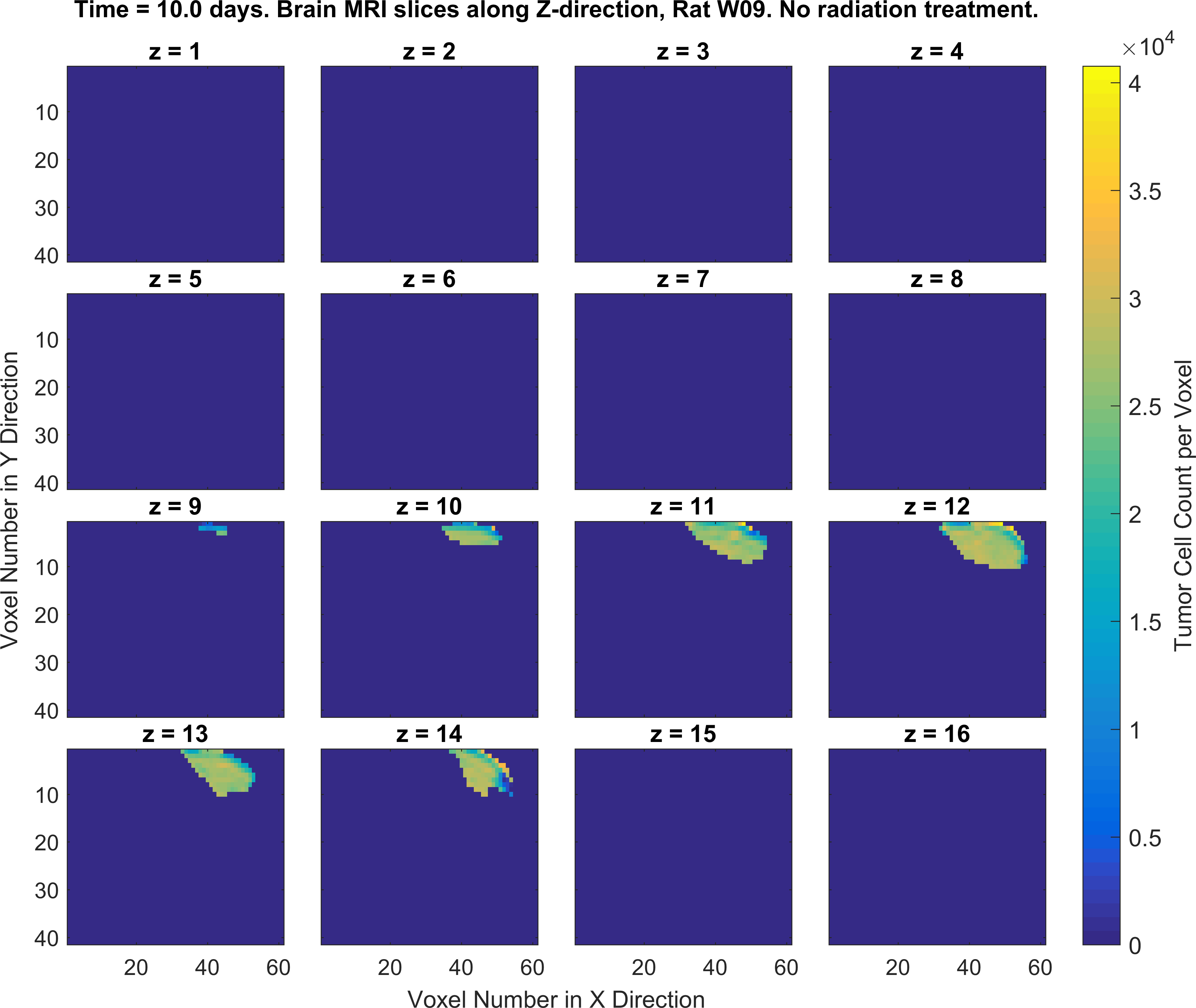
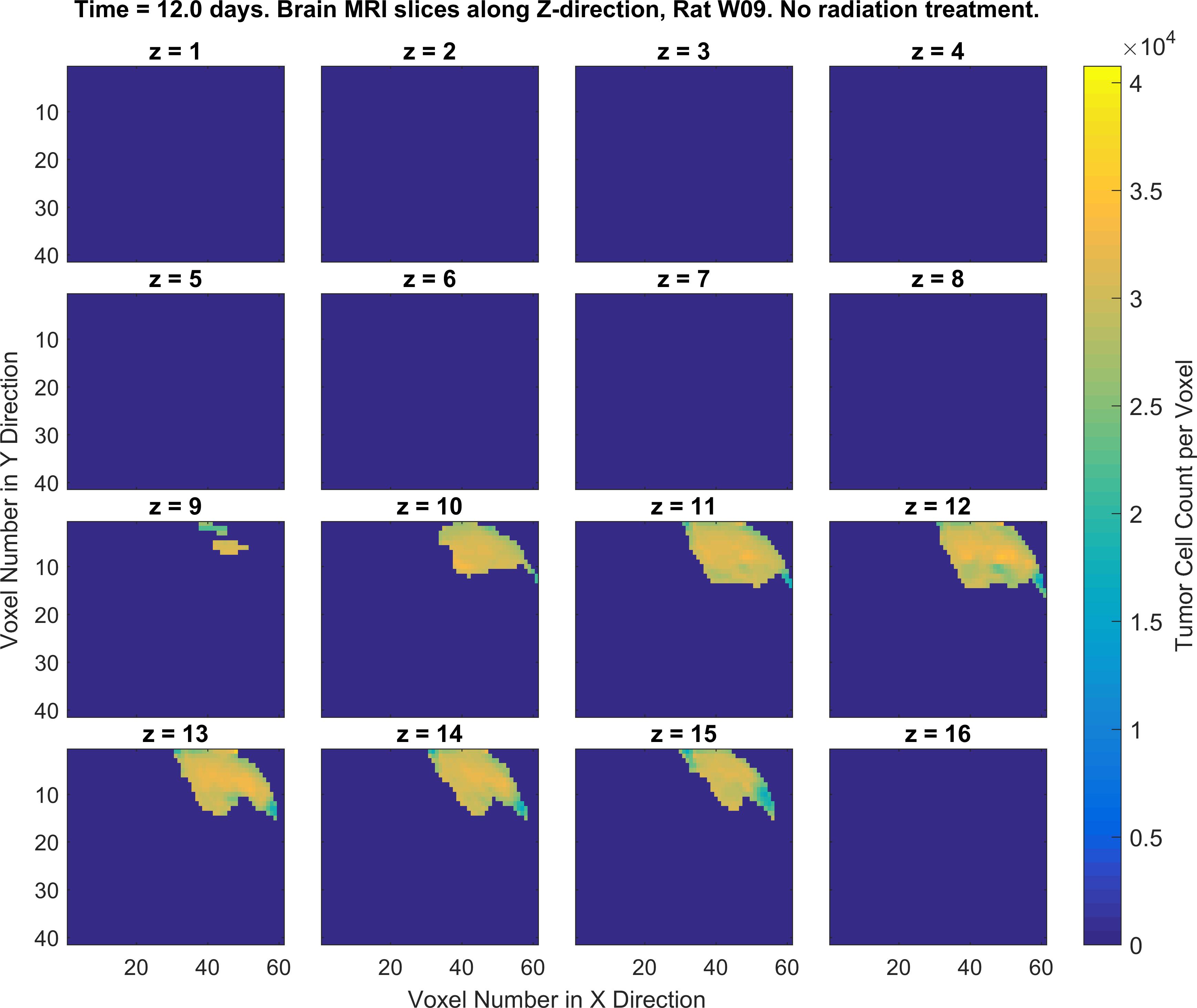
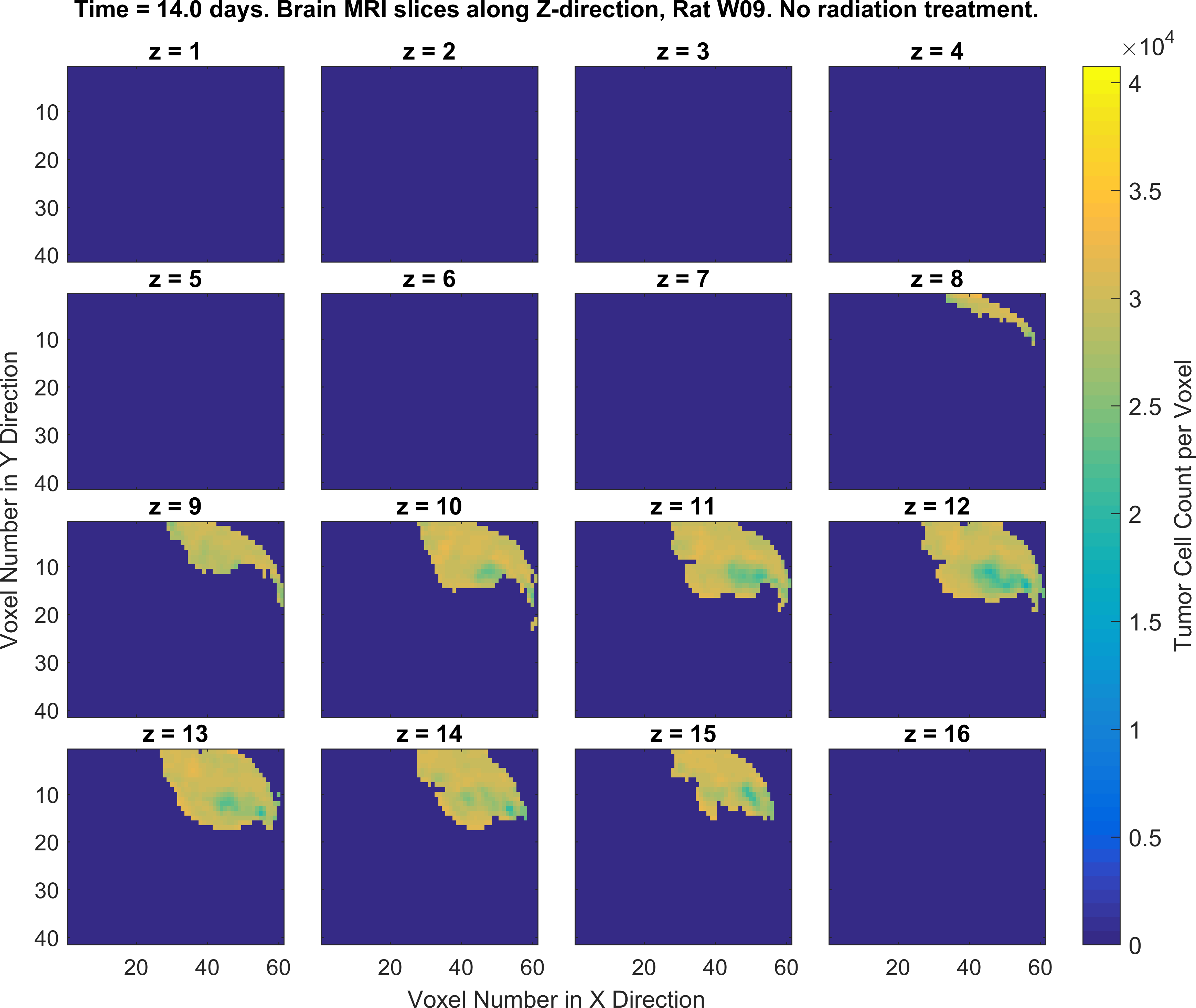
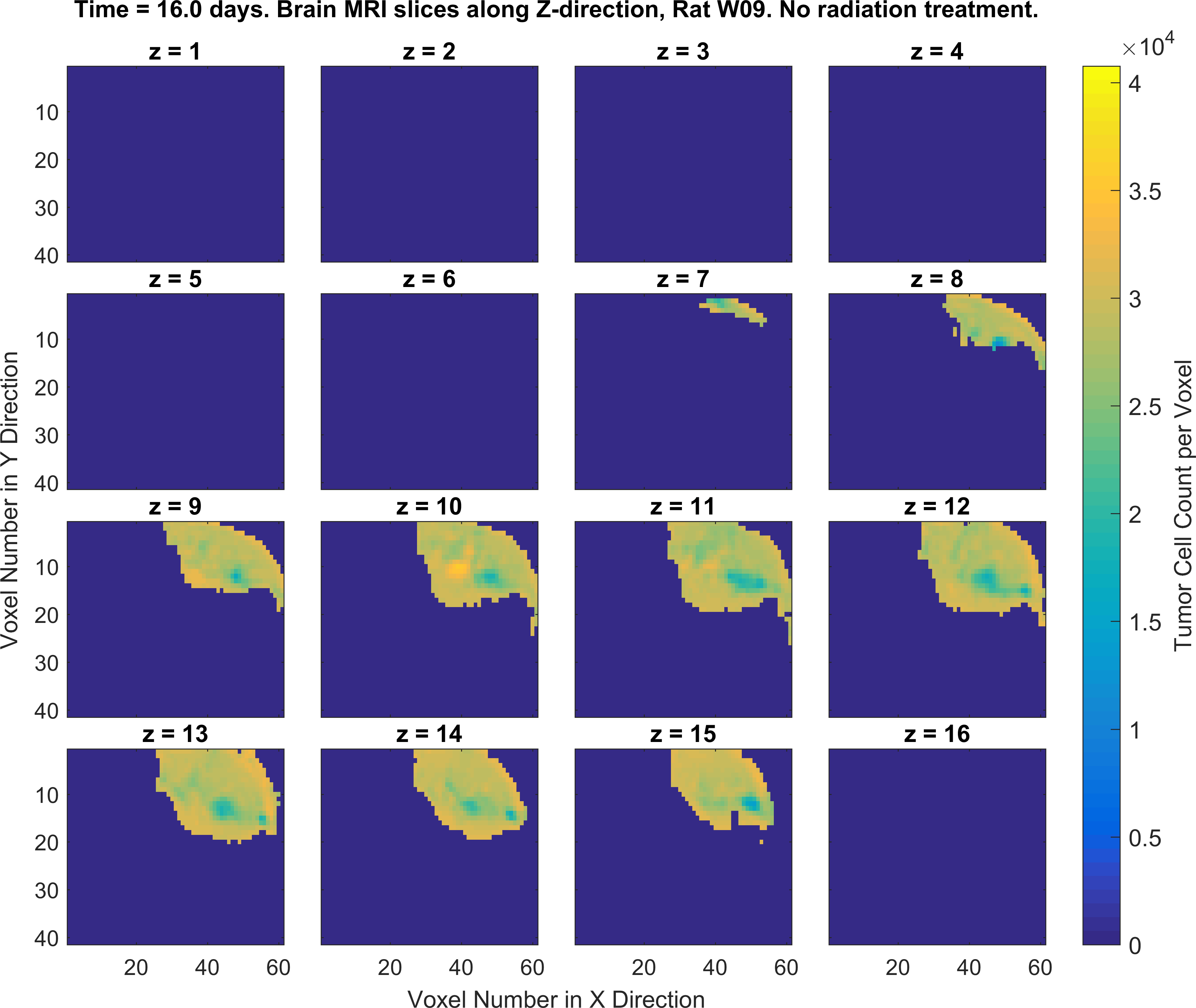
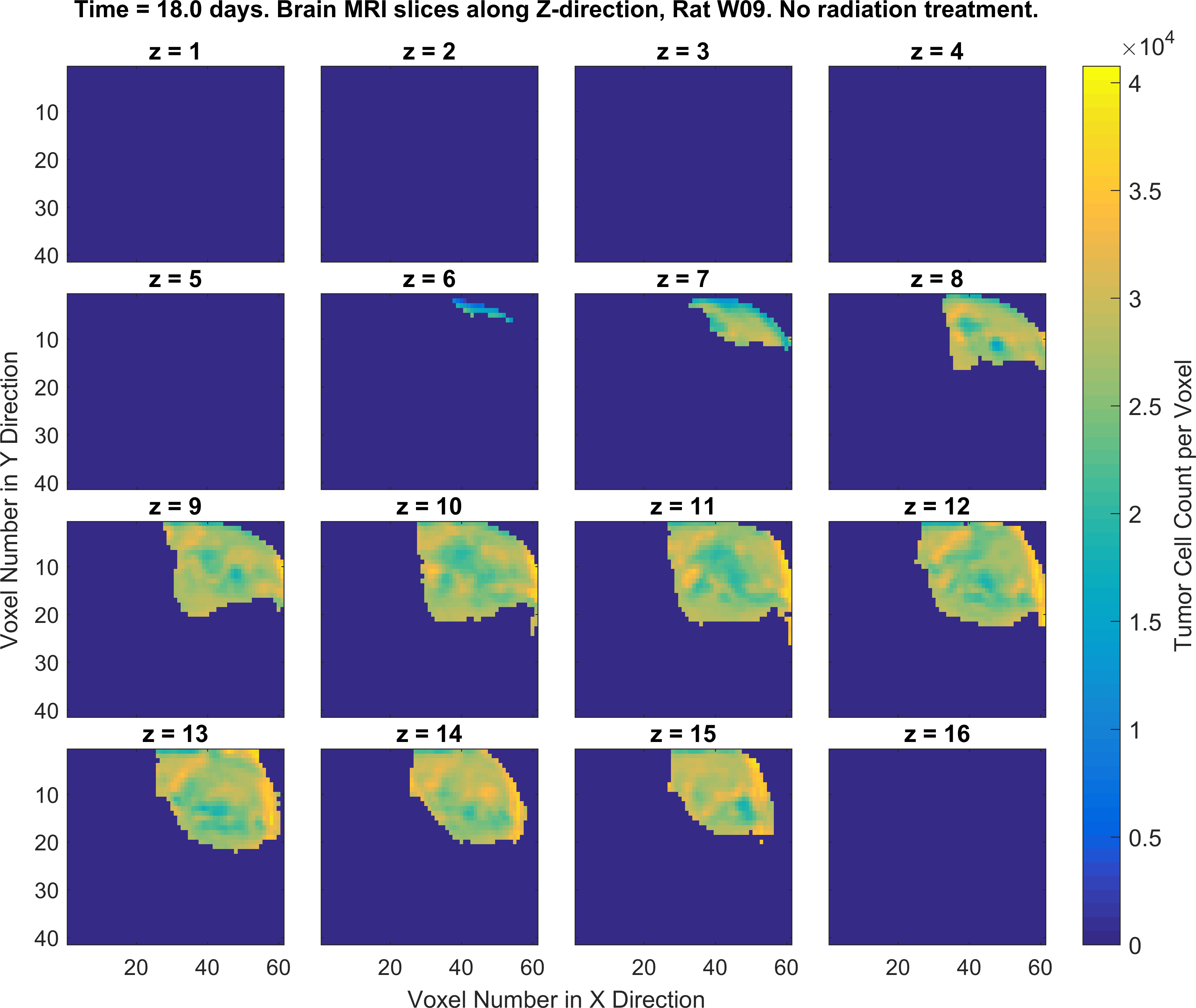
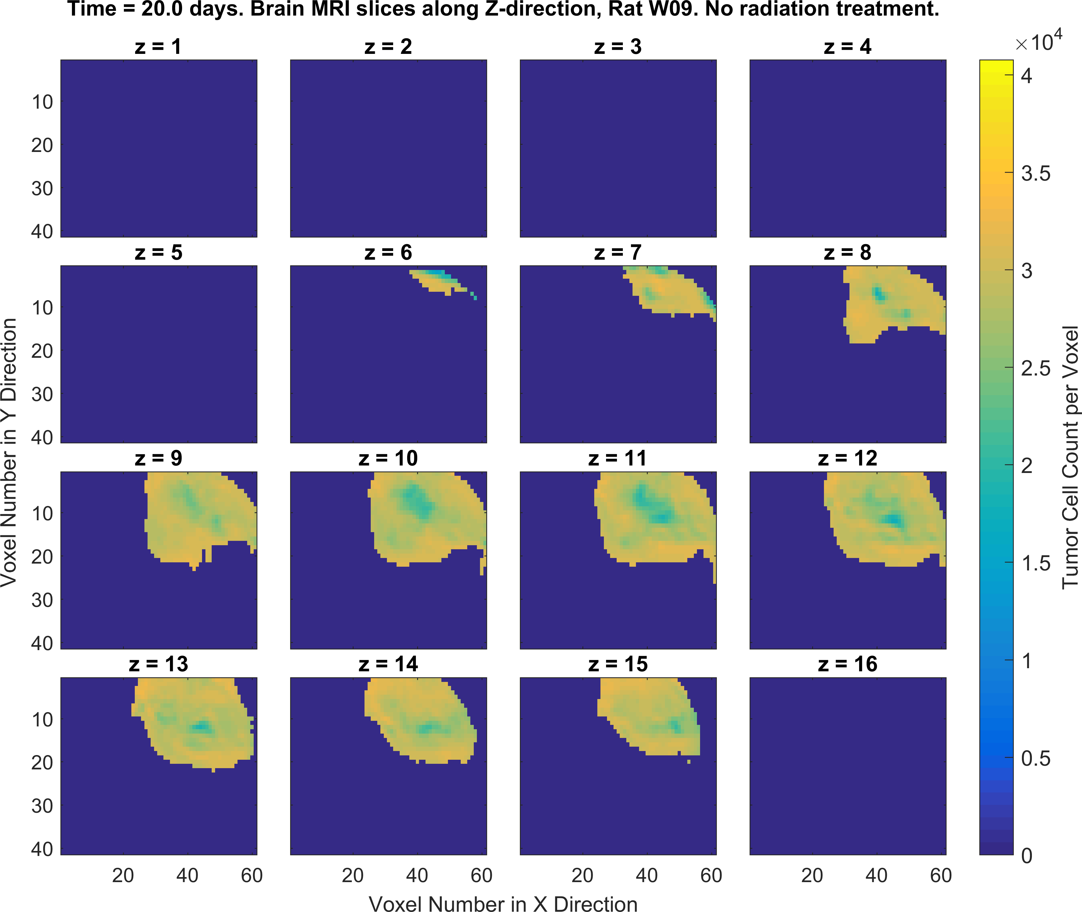
Initially at time $t=0 ~\mathrm{[days]}$, $100,000\pm10,000$ brain tumor cells are injected to the brain of the rat. These cells are then allowed to grow for 10 days. Then starting at day 10, the brain of the rat is imaged using an MRI machine.

Each image results in a 4-dimensional double-precision MATLAB matrix cells(:,:,:,:), corresponding to dimensions cells(y,x,z,time). This data is collected from MRI imaging of the rat’s brain almost every other day for a period of two weeks. For example, cells(:,:,:,1) contains the number of cells at each point in space (y,x,z) at the first time point, or, cells(:,:,10,1) represents a (XY) slice of MRI at $z=1$ and $t=1 [days]$.

Therefore, the vector of times at which we have the number of tumor cells measured would be,

$$Time = [ 0, 10, 12, 14, 16, 18, 20, 22 ] ~,$$

in units of days. Given this data set,

1.  First write a MATLAB/Python script that reads the input MATLAB binary file containing cell numbers at different positions in the rat’s brain measured by MRI, on different days.

2.  Write MATLAB/Python codes that generate a set of figures as similar as possible to the following figures (specific color-codes of the curves and figures do not matter, focus more on the format of the plots and its parts). For this part of the project you will MATLAB plotting functions such as plot(), imagesc() and the concept subplots in MATLAB/Python.

Obtaining the error in tumor cell count

3.  Our assumption here is that the uncertainty in the total number of tumor cells at each time point is given by the number of tumor cells at the boundary of tumor. Therefore, you will have to write a MATLAB code that identifies the boundary of tumor at each time point and then sums over the count cells in all boundary points and uses that as the error in number of tumor cell counts. For this part, you will need MATLAB/Python functions such as bwboundaries() and errorbar(). In the end, you should get and save a figure in your project’s figure folder like the following figure,

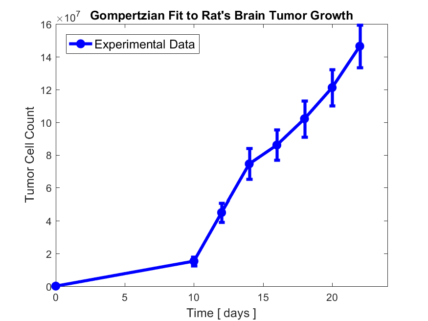
Note that this part of the project is completely independent of the modeling part described in the following section.

The mathematical model of tumor growth

4.  Now our goal is to fit the time evolution of the growth of this tumor, using a mathematical model. To do so, we need to find the best-fit parameters of the model. The mathematical model we will use here is called the Gompertzian growth model. Here, we will use a slightly modified for of the Gompertzian function of the following form,

$$N(t,\lambda,c) = N_0 \times \exp\bigg( \lambda~\bigg[ 1-\exp(-ct) \bigg] \bigg) ~,$$

where $N(t,\lambda,c)$ is the predicted number of tumor cells at time $t$, $N_0$ is the initial number of tumor cells at time $t=0$ days, $\lambda$ is the growth rate parameter of the model, and $c$ is just another parameter of the model. We already know the initial value of the number of tumor cells, $N_0=100,000\pm10,000$. Therefore, we can fix $N_0$ to $100,000$ in the equation of the model given above.

However, we don’t know the values of the parameters $\lambda$ and $c$. Thus, we would like to find their best values given the input tumor cell data using some MATLAB/Python optimization algorithm.

This Gompertzian growth model is called our physical model for this problem, because it describes the physics of our problem (The physics/biology of the tumor growth).

Combining the physical model with a regression model

Now, if our physical model was ideally perfect in describing the data, the curve of the model prediction would pass through all the points in the growth curve plot of the above figure, thus providing a prefect description of data. This is however, never the case, as it is famously said all models are wrong, but some are useful. In other words, the model prediction never matches observation perfectly.

Therefore, we have to seek for the parameter values that can bring the model prediction us as close as possible to data. To do so, we define a statistical model in addition to the physical model described above. In other words, we have to define a statistical regression model (the renowned least-squares method) that gives us the probability $\pi(\log N_{obs}|\log N(t))$ of observing individual data points at each of the given times,

$$\pi(\log N_{obs} | \log N(t,\lambda,c),\sigma) = \frac{1}{\sigma\sqrt{2\pi}} \exp\bigg( - \frac{ \big[ \log N_{obs}(t)-\log N(t,\lambda,c) \big]^2}{2\sigma^2} \bigg) ~,$$

Note that our statistical model given above is a Normal probability density function, with its mean parameter represented by the log of the output of our physical model, $\log N(t,\lambda,c)$, and its standard deviation represented by $\sigma$, which is unknown, and we seek to find it. The symbol $\pi$, whenever it appears with parentheses, like $\pi()$, it means probability of the entity inside the parentheses. However, whenever it appears alone, it means the famous number PI, $\pi\approx 3.1415$.

Why do we use the logarithm of the number of cells instead of using the number of cells directly? The reason behind it is slightly complicated. A simple (but not entirely correct argument) is the following: We do so, because the tumor cell counts at later times become extremely large numbers, on the order of several million cells (For example, look at the number of cells in the late stages of the tumor growth, around $t=20$ days). Therefore, to make sure that we don’t hit any numerical precision limits of the computer when dealing with such huge numbers, we work with the logarithm of the number of tumor cells instead of their true non-logarithmic values.

We have seven data points, so the overall probability of observing all of data $\mathcal{D}$ together (the time vector and the logarithm of the number of cells at different times) given the parameters of the model, $\mathcal{L}(\mathcal{D}|\lambda,c,\sigma)$, is the product of their individual probabilities of observations given by the above equation,

$$\begin{align*} \mathcal{L}(\mathcal{D}|\lambda,c,\sigma) &= \prod_{i=1}^{n=8} \pi(\log N_{obs}(t_i) | \log N(t_i,\lambda,c),\sigma) \\\\ &= \prod_{i=1}^{n=8} \frac{1}{\sigma\sqrt{2\pi}} \exp\bigg( - \frac{ \big[ \log N_{obs}(t_i)-\log N(t_i,\lambda,c) \big]^2}{2\sigma^2} \bigg) ~. \end{align*}$$

Frequently however, you would want to work with $\log\mathcal{L}$ instead of $\mathcal{L}$. This is again because the numbers involved are extremely small often below the precision limits of the computer. So, by taking the logarithm of the numbers, we work instead with number’s exponent, which looks just like a normal number (not so big, not so small). So, by taking the log, the above equation becomes,

$$\begin{align*} \log\mathcal{L}(\mathcal{D}|\lambda,c,\sigma) &= \sum_{i=1}^{n=8} \log \pi( \log N_{obs}(t_i) | \log N(t_i,\lambda,c),\sigma) \\\\ &= \sum_{i=1}^{n=8} \log \bigg[ \frac{1}{\sigma\sqrt{2\pi}} \exp\bigg( - \frac{ \big[ \log N_{obs}(t_i) - \log N(t_i,\lambda,c) \big]^2}{2\sigma^2} \bigg) \bigg] ~. \end{align*}$$

5.  Now the goal is to use an optimization algorithm in MATLAB/Python, such as fminsearch(), to find the most likely set of the parameters of the model $\lambda,c,\sigma$ that give the highest likelihood of obtaining the available data, which is given by the number $\log\mathcal{L}(\mathcal{D}|\lambda,c,\sigma)$ from the above equation. So we want to find the set of parameters for which this number given by the above equation is maximized. You can also use any MATLAB/Python optimization function or method that you wish, to obtain the best parameters.

However, if you use fminsearch(), then note that this function finds the minimum of an input function, not the maximum. What we want is to find the maximum of $\log\mathcal{L}(\mathcal{D}|\lambda,c,\sigma)$. What is the solution then? Very simple. We can multiply the value of $\log\mathcal{L}(\mathcal{D}|\lambda,c,\sigma)$ by a negative, so that the maximum value is converted to minimum. But, note that the position (the set of parameter values) at which this minimum occurs, will remain the same as the maximum position for $\log\mathcal{L}(\mathcal{D}|\lambda,c,\sigma)$.

So, now rewrite your likelihood function above by multiplying its final result (which is just number) by a negative sign. Then you pass this modified function to fminsearch() and you find the optimal parameters. Note that fminsearch() takes as input also a set of initial staring parameter values to initiate the search for the optimal parameters. You can use $(\lambda,c,\sigma) = [10,0.1,1]$ as your starting point given to fminsearch() to search for the optimal values of the parameters.

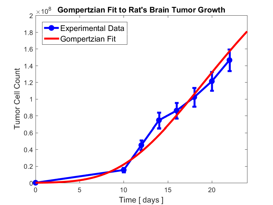
Then redraw the above tumor evolution curve and show the result from the model prediction as well, like the following,

Report also your best fit parameters in a file and submit them with all the figures and your codes to your exam folder repository.