Homework 4: Exceptions, Errors, Vectorization, Visualization

♣ Due Date: Two weeks from the posting date @ 10:30 AM. This homework aims at giving you some experience with data transfer, exceptions and errors, vectorization, and visualization methods in Python and MATLAB. Write your scripts with the corresponding *.py or *.m file names, and add a readme.md file in HW 4 folder of your project if you need to add any additional explanation (Don’t forget to use markdown syntax highlight in your readme file, if needed).

1. Python. Write a simple program named sum.py, that takes in an arbitrary-size list of input floats from the command-line, and prints out the sum of them on the terminal with the following message,

$ python sum.py 1 2 1 23
The sum of 1 2 1 23 is 27.0

Note that you will need to use the Python’s builtin function sum().

2. Python. Similar to the previous problem, write a simple program named sum_via_eval.py, that takes in an arbitrary-size list of input numbers from the command-line, and prints out the sum of them on the terminal, this time using Python’s eval function. The program output should look like the following,

$ python sum.py 1 2 1 23
The sum of 1 2 1 23 is 27

3. Python. Consider this data file. It contains information about the amino-acids in a protein called 1A2T. Each amino-acid in protein is labeled by a single letter. There are 20 amino-acid molecules in nature, and each has a total surface area (in units of Angstroms squared) that is given by the following table,

'A': 129.0
'R': 274.0
'N': 195.0
'D': 193.0
'C': 167.0
'Q': 225.0
'E': 223.0
'G': 104.0
'H': 224.0
'I': 197.0
'L': 201.0
'K': 236.0
'M': 224.0
'F': 240.0
'P': 159.0
'S': 155.0
'T': 172.0
'W': 285.0
'Y': 263.0
'V': 174.0

However, when these amino acids sit next to each other to form a chain protein, they cover parts of each other, such that only parts of their surfaces is exposed, while the rest is hidden from the outside world by other neighboring amino acids. Therefore, one would expect an amino acid that is at the core of a spherical protein would have almost zero exposed surface area.

Now given the above information, write a Python program that takes in two command-line input arguments, one of which is a string containing the path to the above input file 1A2T_A.dssp which contains the partially exposed surface areas of amino acids in protein 1A2T for each of its amino acids, and a second command-line argument which is the path to the file containing output of the code (e.g., it could be ./readDSSP.out). Then,

the code reads the content of this file, and
extracts the names of the amino acids in this protein from the data column inside the file which has the header AA (look at the line number 25 inside the input data file, below AA is the column containing the one-letter names of amino acids in this protein), and
also extracts the partially exposed surface area information for each of these amino acids which appear in the column with header ACC, and
then uses the above table of maximum surface area values to calculate the fractional exposed surface area of each amino acid in this protein (i.e., for each amino acid, fraction_of_exposed_surface = ACC / maximum_surface_area_from_table), and
finally for each amino acid in this protein, it prints the one-letter name of the amino acid, its corresponding partially exposed surface area (ACC from the input file), and its corresponding fractional exposed surface area (name it RSA) to the output file given by the user on the command line.
On the first column of the output file, the code should also write the name of the protein (which is basically the name of the input file 1A2T_A) on each line of the output file. Note that your code should extract the protein name from the input filename (by removing the file extension and other unnecessary information from the input command line string). Here is an example output of the code.
Your code should also be able to handle an error resulting from less or more than 2 input command line arguments. That is, if the number of input arguments is 3 or 1, then it should input the following message on screen and stop.

$ ./readDSSP.py ./1A2T_A.dssp


Usage:
      ./readDSSP.py <input dssp file> <output summary file>

Program aborted.

or,

$ ./readDSSP.py ./1A2T_A.dssp ./readDSSP.out amir


Usage:
      ./readDSSP.py <input dssp file> <output summary file>

Program aborted.

To achieve the above goal, you will have to create a dictionary from the above table, with amino acid names as the keys, and the maximum surface areas as the corresponding values. Name your code readDSSP.py and submit it to your repository.

Write your code in such a way that it checks for the existence of the output file. If it already exists, then it does not remove the content of the file, whereas, it appends new data to the existing file. therwise, if the file does not exist, then it creates a new output file as requested by the user. To do so, you will need to use os.path.isfile function from module os.

ATTENTION: Note that in some rows instead of a one-letter amino acid name, there is !. In such cases, your code should be able to detect the abnormality and skip that row, because that row does not contain amino acid information.

4. MATLAB. Solve the same problem as in 3, except that you don’t need to read the arguments (i.e., filenames) from the command line. Instead, implement your script as a MATLAB function.

5. Python. Consider the simplest program for evaluating the formula $y(t) = v_0t-\frac{1}{2}gt^2$,

v0 = 3; g = 9.81; t = 0.6
y = v0*t - 0.5*g*t**2
print(y)

(A) Write a program that takes in the above necessary input data ($t$,$v_0$) as command line arguments.

(B) Extend your program from part (A) with exception handling such that missing command-line arguments are detected. For example, if the user has entered enough input arguments, then the code should raise IndexError exception. In the except IndexError block, the code should use the input function to ask the user for the missing input data.

(C) Add another exception handling block that tests if the $t$ value read from the command line, lies between $0$ and $2v_0/g$. If not, then it raises a ValueError exception in the if block on the legal values of $t$, and notifes the user about the legal interval for $t$ in the exception message.

Here are some example runs of the code,

$ ./projectile.py
Both v0 and t must be supplied on the command line
v0 = ?
5
t = ?
4
Traceback (most recent call last):
  File "./projectile.py", line 17, in <module>
    'must be between 0 and 2v0/g = {}'.format(t,2.0*v0/g))
ValueError: t = 4.0 is a non-physical value.
must be between 0 and 2v0/g = 1.019367991845056

$ ./projectile.py
Both v0 and t must be supplied on the command line
v0 = ?
5
t = ?
0.5
y = 1.27375

$ ./projectile.py 5 0.4
y = 1.2151999999999998

$ ./projectile.py 5 0.4 3
y = 1.2151999999999998

6. Python. Consider the function Newton,

def Newton(f, dfdx, x, eps=1E-7, maxit=100):
    if not callable(f): raise TypeError( 'f is %s, should be function or class with __call__' % type(f) )
    if not callable(dfdx): raise TypeError( 'dfdx is %s, should be function or class with __call__' % type(dfdx) )
    if not isinstance(maxit, int): raise TypeError( 'maxit is %s, must be int' % type(maxit) )
    if maxit <= 0: raise ValueError( 'maxit=%d <= 0, must be > 0' % maxit )
    n = 0 # iteration counter
    while abs(f(x)) > eps and n < maxit:
        try:
            x = x - f(x)/float(dfdx(x))
        except ZeroDivisionError:
            raise ZeroDivisionError( 'dfdx(%g)=%g - cannot divide by zero' % (x, dfdx(x)) )
        n += 1
    return x, f(x), n

This function is supposed to be able to handle exceptions such as divergent iterations, and division-by-zero. The latter error happens when dfdx(x)=0 in the above code. Write a test code that ensures the above code is able to correctly identify a division-by-zero exception and raise the correct assertionError.
(Hint: To do so, you need to consider a test mathematical function as input to Newton. One example could be $f(x)=\cos(x)$ with a starting search value $x=0$. This would result in derivative value $f’(x=0)=-\sin(x=0)=0$, which should lead to a ZeroDivisionError exception. Now, write a test function test_Newton_div_by_zero that can explicitly handle this exception by introducing a boolean variable success that is True if the exception is raised and otherwise False.)

7. Reading scientific data from web using Python/MATLAB. Consider the following webpage address https://www.cdslab.org/ICP2017F/homework/5-problems/swift/bat_time_table.html. This is an data table (in HTML language) containing data from NASA’s Swift satellite. Each row in this table represents information about a Gamma-Ray Burst (GRB) detection that Swift has made in the past years. Now, corresponding to each of event IDs, there (might) exist files that contain some attributes of these events which we wish to plot and understand their behavior. For example, for the first event in this table, contains a data file which is hidden in a directory on this website here. For each event in this table, there is likely one such table hidden in this web directory.

Our goal in this question is to fetch all these files from the website and save them locally in our own computer. Then read their contents one by one and plot the two columns of data in all of them together.

(A) Write a script named fetchDataFromWeb.* (with the star * indicating the arbitrary choice of your own language) that uses this web address: https://www.cdslab.org/ICP2017F/homework/5-problems/triggers.txt to read a list of all GRB events and then writes the entire table of triggers.txt to a local file with the same name on your device. For this purpose, you will need some built-in or library functionality to read the contents of a web page, such as webread() in MATLAB or the package urllib.request in Python (or some other libraries).

(B) Now, add to your script another set of commands that uses the event IDs stored in this file, to generate the corresponding web addresses like: https://www.cdslab.org/ICP2017F/homework/5-problems/swift/GRB00745966_ep_flu.txt. Then it uses the generated web address to read the content of the page and store it in a local file on your device with the same name as it is stored on the webpage (for example, for the given webpage, the filename would be GRB00745966_ep_flu.txt). Note: Some of the web addresses for the given event IDs do not exist. Therefore, you should use an exception-handling construct such as MATLAB’s try-catch or Python’s try-except construct to avoid runtime errors in your code.

(C) Now write another script named plotDatafromFile.m, that reads all of these files in your directory, one by one, and plots the content of all of them together, on a single scatter plot like the following,

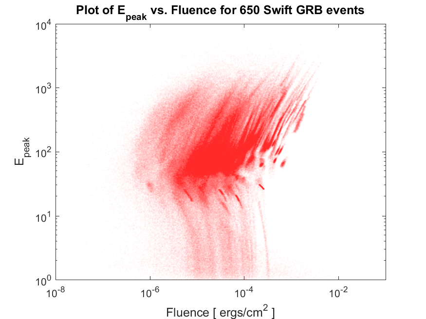
Note again that some the data files stored on your computer are empty and some others have useless data if data in the second column of the file is larger than 0. So you will have to write your script in such a way that it checks for non-emptiness of the file (that is, the file does indeed contain some numerical data) as well as the negativity of the values in the column of data in each file. For example, you could check for the negativity of the values in MATLAB using function all(data[:,1]<0.0) assuming that data is the variable containing the information read from the file.

Once you have done all these checks, you have to do one final manipulation of data, that is, the data in these files on the second column is actually the log of data, so have to get the exp() value to plot it (because the plot in the figure above is a log-log plot and we want to exactly regenerate it). To do so in MATLAB, for example, you could simply use the following,

data[:,2] = exp(data[:,2]);

as soon as you read from the file, and then finally you make a scatter plot of all data using MATLAB scatter plot. At the end, you will have to set a title for your plot as well and label the axes of the plot, and save your plot using MATLAB’s built-in function saveas(). In order to find out how many files you have plotted in the figure, you will have to define a variable counter which increases by one unit, each time a new non-empty negative-second-column data file is read and plotted.

8. Simulating a fun Monte Carlo game. Suppose you’re on a game show, and you’re given the choice of three doors:

Behind one door is a car; behind the two others, goats. You pick a door, say No. 1, and the host of the show opens another door, say No. 3, which has a goat.

He then says to you, “Do you want to pick door No. 2?”.

Question: What would you do? Is it to your advantage to switch your choice from door 1 to door 2? Is it to your advantage, in the long run, for a large number of game tries, to switch to the other door?

Now whatever your answer is, I want you to check/prove your answer by a Monte Carlo simulation of this problem. Make a plot of your simulation for nExperiments=100000 repeat of this game, that shows, in the long run, on average, what is the probability of winning this game if you switch your choice, and what is the probability of winning, if you do not switch to the other door.

Hint: I strongly urge you to attend the lectures this week in order to get help for this question.

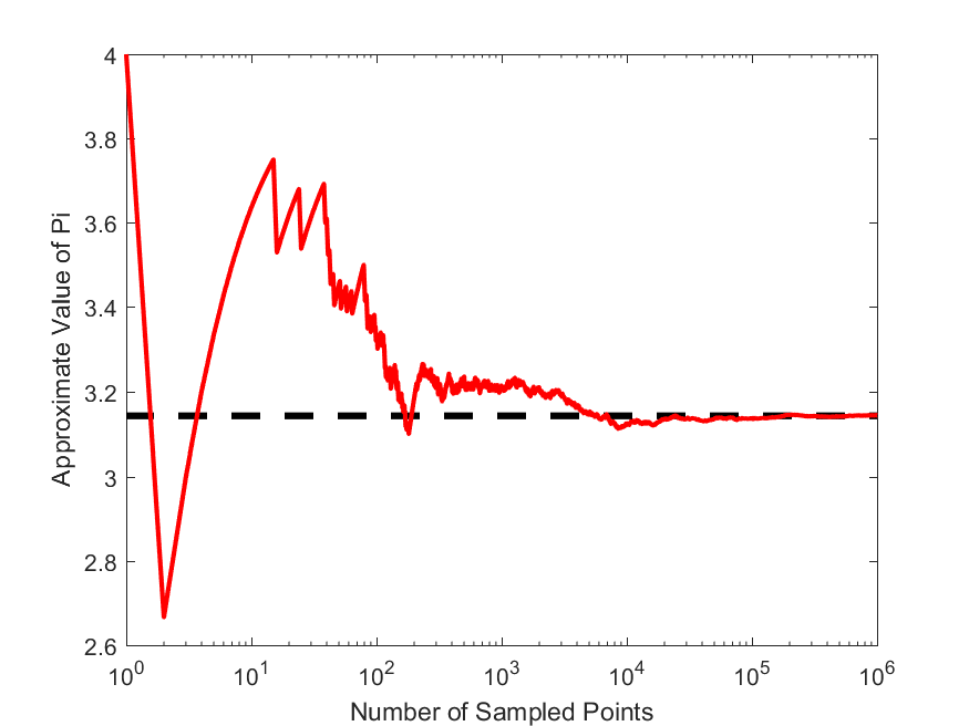
9. Monte Carlo approximation of the number $\pi$. Suppose we did not know the value of $\pi$ and we wanted to estimate its value using Monte Carlo methods. One practical approach is to draw a square of unit side, with its diagonal opposite corners extending from the coordinates origin $(0,0)$ to $(1,1)$. Now we try to simulate uniform random points from inside of this square by generating uniform random points along the $X$ and $Y$ axes, i.e., by generating two random uniform numbers (x,y) from the range $[0,1]$.

Now the generated random point $P$ has the coordinate $(x,y)$, so we can calculate its distance from the coordinate origin. Now suppose we also draw a quarter-circle inside of this square whose radius is unit and is centered at the origin $(0,0)$. The ratio of the area of this quarter-circle, $S_C$ to the area of the area of the square enclosing it, $S_S$ is,

$\frac{S_C}{S_S} = \frac{\frac{1}{4}\pi r^2}{r^2} = \frac{1}{4}\pi$

This is because the area of the square of unit sides, is just 1. Therefore, if we can somehow measure the area of the quarter $S_C$, then we can use the following equation, to get an estimate of $\pi$,

$\pi = 4S_C$

In order to obtain, $S_C$, we are going to throw random points in the square, just as described above, and then find the fraction of points, $f=n_C/n_{\rm total}$, that fall inside this quarter-circle. This fraction is related to the area of the circle and square by the following equation,

$f=\frac{n_C}{n_{\rm total}} = \frac{S_C}{S_S}$

Therefore, one can obtain an estimate of $\pi$ using this fraction,

$\pi \approx 4\frac{n_C}{n_{\rm total}}$

Now, write a MATLAB script, that takes in the number of points to be simulated, and then calculates an approximate value for $\pi$ based on the Monte Carlo algorithm described above. Write a second function that plot the estimate of $\pi$ versus the number of points simulated, like the following,

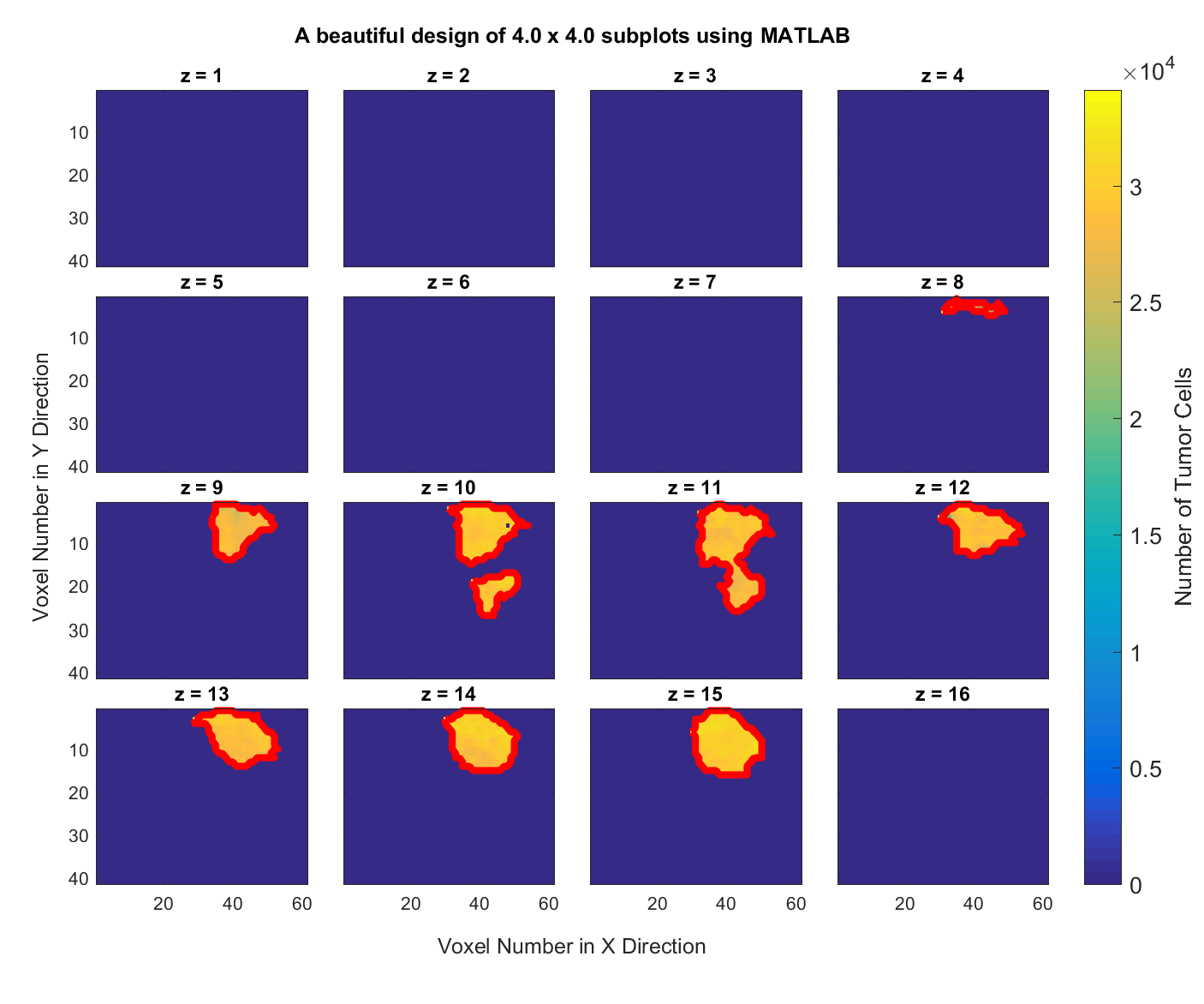
10. Subplots in MATLAB. Consider this MATLAB data file data3D.mat which contains a 3-dimensional $41\times 61\times 16$ matrix of the brain of a rat. Write a MATLAB script that creates and saves a graph of all $X-Y$ information for the 16 slices along the z axis like the following.

Hint: Start from this MATLAB script that I have written for you. Play with all the options to understand what they do and see their effects on the resulting plot. This script should generate the following figure for you.

11. MATLAB. Getting the boundary of objects in images.. Consider the same dataset as in the previous problem. Write a MATLAB script that delineates the boundary of the tumor in all of the subplots and generates a figure with the tumor boundary highlighted, like the following graph.

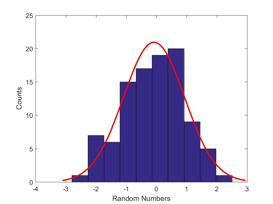
12. MATLAB. Regression: obtaining the most likely mean and standard deviation of a set of Standard Normally Distributed Random Variables. Consider this dataset, Drand.mat, which contains a set of random numbers. Let’s make a hypothesis with regards to this dataset: We assume that this dataset is well fit by a Gaussian distribution. But, we don’t know the values of the two parameters (mean and standard deviation) of this Normal (Gaussian) distribution. Therefore, write a MATLAB script that constructs an objective function (similar to what we are planning to do for the mathematical modeling section of the project) and then uses MATLAB’s built-in function, fminsearch(), to find the most likely values of the mean and standard deviation of this Gaussian distribution. Here is a best-fit Gaussian distribution using the most likely parameters to the histogram of this dataset.

Hints: Our hypothesis is that the data in this histogram comes from a standard Normal distribution with a fixed mean ($\mu$) and standard deviation ($\sigma$). For the moment, let’s assume that we know the values of these two parameters. Then if all of these points, $D$, come from the normal distribution with the given $(\mu,\sigma)$, then the probability of all them coming from the normal distribution with these parameter values can be computed as,

$\pi\big(\boldsymbol D\big|\mu,\sigma\big) = \prod^{N=100}_{i=1} \frac{1}{2\pi\sigma^2}\exp\bigg( -\bigg[ \frac{\boldsymbol D(i)-\mu}{\sqrt{2}\sigma} \bigg]^2 \bigg) ~~,$

where the symbol $\pi$ to the left of equality means probability (but note that $\pi$ on the right hand side of the euqation stands for the number $\pi=3.14\ldots$, and $D(i)$ refers to the $i$th point in the sample of points. Since probabilities are always extremely small numbers, it is always good to work with their log() values instead of their raw values (can you guess why?). Therefore, we could take the log of the above equation to write it as,

$\log\pi\big(\boldsymbol D\big|\mu,\sigma\big) = \sum^{N=100}_{i=1} - \log\big(2\pi\sigma^2\big) - \bigg[ \frac{\boldsymbol D(i)-\mu}{\sqrt{2}\sigma} \bigg]^2 ~~,$

Now our goad is to construct this function (let’s name it getLogProbNorm()) and pass it to MATLAB’s built-in function fminsearch() in order to find the most likely $(\mu,\sigma)$ that leads to the highest likelihood value (the maximum of the above equation). Here is one last tip: Note that fminsearch() minimizes functions, but we want to maximize getLogProbNorm(), instead of minimizing it. What change could you make to this function to make it work with fminsearch()? Name your main script findBestFitParameters.m. Now when you run your script it should call fminsearch() and then output the best-fit parameters like the following,

>> findBestFitParameters
mu: -0.082001 , sigma: 1.0043

Start your parameter search via fminsearch() with the following values: $[\mu,\sigma] = [1,10]$.

Homework 4: Exceptions, Errors, Vectorization, Visualization

Amir Shahmoradi

Comments