MATLAB visualization and plotting capabilities are among the most powerful features of MATLAB and a major driver of MATLAB popularity, to the extent that many Python packages, the most prominent of which are matplotlib have been inspired by MATLAB plotting syntax and capabilities.
Curve plotting in MATLAB
One of the most useful methods of outputting the results of your research and MATLAB projects is plotting. Here, we will only review some of the most important and most useful plotting capabilities in MATLAB.
Plotting simple 2D data
One of the most widely used MATLAB plotting functions is plot(). With this function, plotting x-y data is as simple as it can be. All you need to have is a dataset consisting of X and Y vectors,
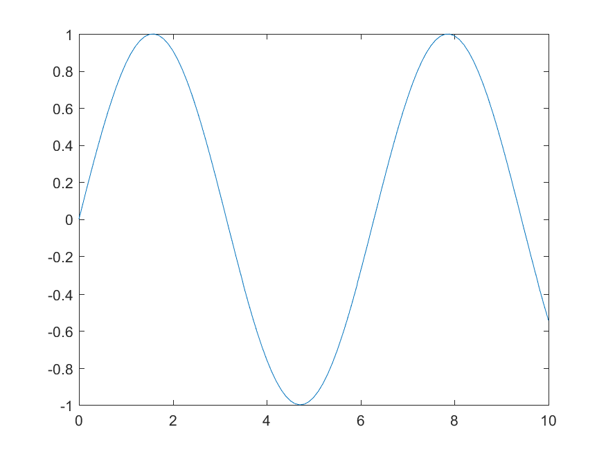
>> X = 0:0.1:10;
>> plot(X,sin(X));
This will open the following MATLAB figure page for you in the MATLAB environment,
You could also save this figure in almost any format you wish using save() function,
>> saveas(gcf,'sin.png')
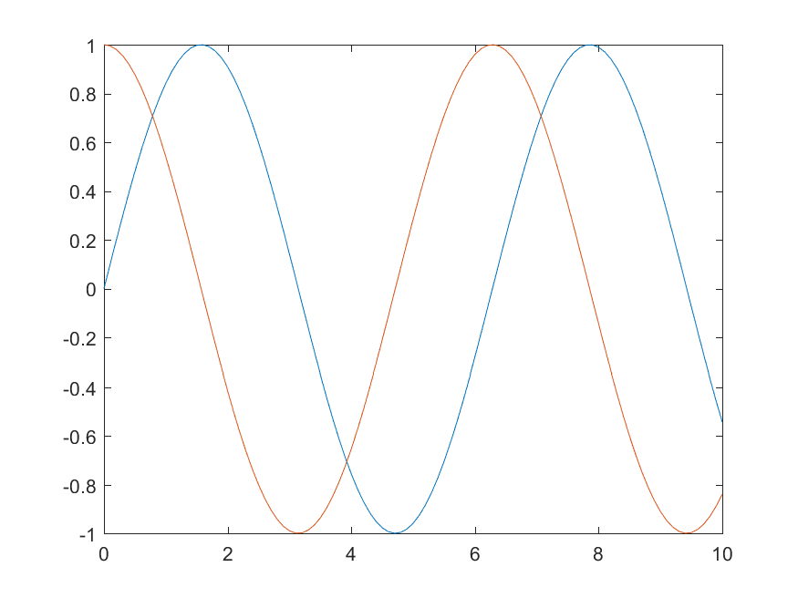
Here, gcf refers tothe current figure handle in MATLAB environment. If you wish to add new data to this plot, you could use hold on; command,
>> hold on;
>> plot(X,cos(X));
>> saveas(gcf,'sinCos.png')
This will save the following figure for you, on your local device,
Annotating and decorating your MATLAB plots
Things you can do with MATLAB plotting functions are virtually endless, and there is no way we could cover all of them here in this course. Nevertheless, here are a few useful commands that help you decorate your plots. For example, you could add a plot title as well as X-axis and Y-axis labels to your plots by,
>> title('A simple plot of Sin(x) and Cos(X)', 'fontsize', 12)
>> xlabel('X value', 'fontsize', 13);
>> ylabel('Y value', 'fontsize', 13);
Also we could add legends to the plot, explaining what each line represents,
>> legend( { 'Sin(X)' , 'Cos(X)' } , 'fontsize' , 13 , 'location' , 'southwest' );
Note that the fontsize keyword is not necessary. You could simply omit it and MATLAB’s default font size will be used instead.
You could also change the line-width of the borders of the plot, for example, by,
>> set( gca , 'linewidth' , 3 );
Here, gca is a MATLAB keyword that refers to the current active plot in the current active figure. If you wanted to thicken the curve lines themselves, you could simple add the 'linewidth' keyword when calling plot(), along with the desired line width value. You could also determine the line color using color keyword followed by the desired color,
>> hold off; % this closes access to the old figure
>> figure() % this creates a new figure handle
>> plot(X,sin(X),'linewidth',3, 'color', 'blue');
>> hold on;
>> plot(X,cos(X),'linewidth',3, 'color', 'red');
>> legend( { 'Sin(X)' , 'Cos(X)' } , 'fontsize' , 13 , 'location' , 'southwest' );
>> title('A simple plot of Sin(x) and Cos(X)', 'fontsize', 12)
>> xlabel('X value', 'fontsize', 13);
>> ylabel('Y value', 'fontsize', 13);
>> set( gca , 'linewidth' , 3 );
>> saveas(gcf,'sinCosDecorated.png')
This will generate the following figure and save it to your local hard drive,
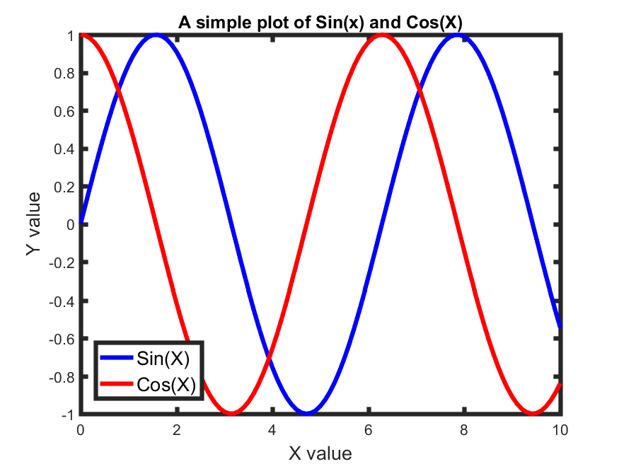
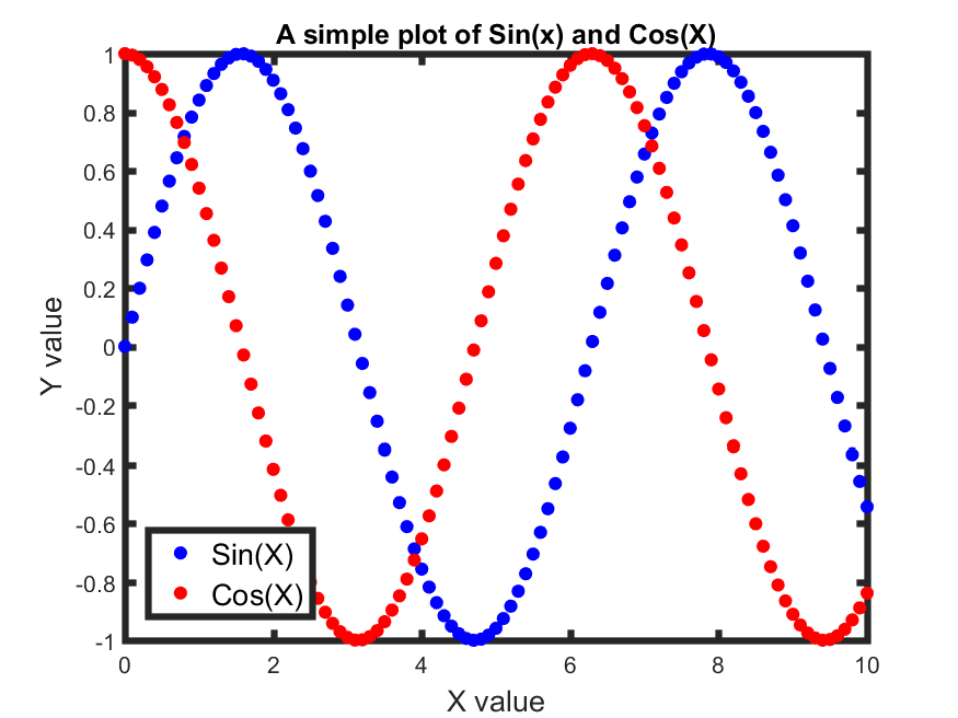
You can also plot the data using different line/ point styles. For example, to plot the same data using points instead of lines, all you need to do, is to add the '.' string to your plot() functions, indicating that you want a scatter plot, instead of line plot,
>> figure() % this creates a new figure handle
>> plot(X,sin(X), '.', 'color', 'blue', 'markersize', 20);
>> hold on;
>> plot(X,cos(X), '.', 'color', 'red', 'markersize', 20);
>> legend( { 'Sin(X)' , 'Cos(X)' } , 'fontsize' , 13 , 'location' , 'southwest' );
>> title('A simple plot of Sin(x) and Cos(X)', 'fontsize', 12)
>> xlabel('X value', 'fontsize', 13);
>> ylabel('Y value', 'fontsize', 13);
>> set( gca , 'linewidth' , 3 );
>> saveas(gcf,'sinCosDecoratedScatter.png')
which will produce and save the following plot,
To learn more about fantastic things you can do with MALTAB plotting functions, see this page.
Other more complex plotting functions in MATLAB
MATLAB, as said above, has a tremendous set of plotting functions, which make it an ideally suited programming language for scientific research. We will learn how to use some of these functions in homework 5. Here on this page, you can find a long list of MATLAB plotting functions and types of plots that you can draw using MATLAB.
Closing figures and plots in MATLAB
for closing the current active figure in MATLAB, you could simply use close(gcf). Here, gcf refers to the current active figure handle. To close all open figures, simply type close all;.