Values in MATLAB

Values and their types in MATLAB

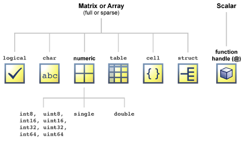
Values are one of the most fundamental entities in programming. Like any other language, a value in MATLAB can be of different types, most importantly Numeric (plain integer, long integer, float (real number), complex), Boolean (logical) which is a subtype of Numeric, or char (string), and many more. Each value type in MATLAB is a class. We will get to what classes are, at the end of the semester. For now, all you need to know is that there 6 main data types (in addition to function handles).

Numeric and logical values in MATLAB

The following are a few example arithmetic operations with values in MATLAB. You can perform very simple arithmetic on the MATLAB command line, and the result immediately by pressing enter.

2 + 5 % Just typing some comment on the MATLAB command line. Anything after % is a comment and will be ignored.

ans =
     7

2 - 7 % difference

ans =
    -5

2 * 7 % product

ans =
    14

true % logical true value

ans =
     1

false % logical false value

ans =
     0

Obtaining the type (class) of values

You can use the MATLAB’s built-in function class to get the type of a value in MATLAB (Of course, this is somewhat obvious and redundant for a value input as we already readily know the type of a value).

class(2*7) % class function gives you the type of the input object to function "class"

ans =
double

class('This is a MATLAB string (char)') % a char value in MATLAB

ans =
char

class("This is a MATLAB string") % Note that you cannot use quotation marks for representing string values.

 class("This is a MATLAB string") % Note that you cannot use quotation marks for representing string values.
       ↑
Error: The input character is not valid in MATLAB statements or expressions.

class(1)

ans =
double

class(class(1))

ans =
char

class(true)

ans =
logical

class(false)

ans =
logical

vector and matrix values

Vectors and matrices are used to represent sets of values, all of which have the same type. A matrix can be visualized as a table of values. The dimensions of a matrix are $rows \times cols$, where $rows$ is the number of rows and $cols$ is the number of columns of the matrix. A vector in MATLAB is equivalent to a one-dimensional array or matrix.

Creating row-wise and column-wise vectors

Use , or space to separate the elements of a row-wise vector.

[1 2 3 4] % a space-separated row vector

ans =
     1     2     3     4

class([1 2 3 4])

ans =
double

[1, 2, 3, 4] % a comma-separated row vector

ans =
     1     2     3     4

class([1, 2, 3, 4])

ans =
double

[1; 2; 3; 4] % a column vector

ans =
     1
     2
     3
     4

class([1; 2; 3; 4])

ans =
double

Creating matrix values

Use ; to separate a row of the matrix from the next.

[1,2,3,4;5,6,7,8;9,10,11,12] % a 3 by 4 matrix

ans =
     1     2     3     4
     5     6     7     8
     9    10    11    12

Cells and tables

Matrices and vectors can only store numbers in MATLAB. If one needs a more general array representation for a list of strings for example, then one has to use cells or tables.

Cell array values

Cell arrays are array entities that can contain data of varying types and sizes. A cell array is a data type with indexed data containers called cells, where each cell can contain any type of data. Cell arrays commonly contain either a list of text strings, combinations of text and numbers, or numeric arrays of different sizes. Refer to sets of cells by enclosing indices in smooth parentheses, (). Access the contents of cells by indexing with curly braces, {}. Also, to define a cell, use {} like the following notation,

{'Hi', ' ', 'World!'} % a cell array of strings

ans = 
    'Hi'    ' '    'World!'

class({'Hi', ' ', 'World!'})

ans =
cell

{'Hi', 1, true, 'World!'}

ans = 
    'Hi'    [1]    [1]    'World!'

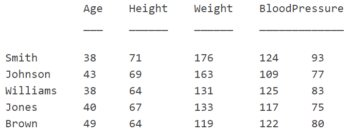
Table values

MATLAB tables are arrays in a tabular form whose named columns can have different types. MATLAB’s Table is a data type suitable for column-oriented or tabular data that is often stored as columns in a text file or a spreadsheet. Tables consist of rows and column-oriented variables. Each variable in a table can have a different data type and a different size with the one restriction that each variable must have the same number of rows.

Later on, we learn more about Tables and Cells in MATLAB, once we introduce MATLAB variables.

Value coercion in MATLAB

Value coercion is the implicit process by which the MATLAB interpreter/compiler automatically converts a value of one type into a value of another type when that second type is required by the surrounding context. For example,

class(int32(1.0)) % int32 gives a 32-bit (4-byte) integer.

ans =
int32

int32(2.0) * int32(1.0) % Note that the product of two integers, is integer.

ans =
           2

class(ans)

ans =
int32

int32(1.0) * 2.5 % Note that the product of float and integer is coerced into an integer!

ans =
           3

class(ans)

ans =
int32

int32(1.0) / 2.5 % Note that the division of float and integer, is coerced into an integer.

ans =
           0

2.0 / 7 % floating point division with float result

ans =
    0.2857

true + 1 % logical and double are coerced into double

ans =
     2

class(true + 1)

ans =
double

However, note that,

true + int32(1) % you cannot combine logical with integer

Error using  + 
Integers can only be combined with integers of the same class, or scalar doubles.

true + false

ans =
     1

true * false

ans =
     0

true / false

Undefined operator '/' for input arguments of type 'logical'.

Some further useful MATLAB commands

MATLAB has a built-in function called format that can modify the output style of MATLAB on the command line. For example,

2/5

ans =
    0.4000

format long
2/5

ans =
   0.400000000000000

format short
2/5

ans =
    0.4000

format loose
2/5

ans =

    0.4000

format compact
2/5

ans =
    0.4000

Here is a complete list of options that format can take,