Monte Carlo approximation of the number Pi

Problem

Suppose we did not know the value of $\pi$ and we wanted to estimate its value using Monte Carlo methods. One practical approach is to draw a square of unit side, with its diagonal opposite corners extending from the coordinates origin $(0,0)$ to $(1,1)$. Now we try to simulate uniform random points from inside of this square by generating uniform random points along the $X$ and $Y$ axes, i.e., by generating two random uniform numbers (x,y) from the range $[0,1]$.

Now the generated random point $P$ has the coordinate $(x,y)$, so we can calculate its distance from the coordinate origin. Now suppose we also draw a quarter-circle inside of this square whose radius is unit and is centered at the origin $(0,0)$. The ratio of the area of this quarter-circle, $S_C$ to the area of the square enclosing it, $S_S$ is,

\[\frac{S_C}{S_S} = \frac{\frac{1}{4}\pi r^2}{r^2} = \frac{1}{4}\pi\]

This is because the area of the square of unit-length sides is just 1. Therefore, if we can somehow measure the area of the quarter $S_C$, then we can use the following equation, to get an estimate of $\pi$,

\[\pi = 4S_C\]

To obtain, $S_C$, we are going to throw random points in the square, just as described above, and then find the fraction of points, $f=n_C/n_{\rm total}$, that fall inside this quarter-circle. This fraction is related to the area of the circle and square by the following equation,

\[f=\frac{n_C}{n_{\rm total}} = \frac{S_C}{S_S}\]

Therefore, one can obtain an estimate of $\pi$ using this fraction,

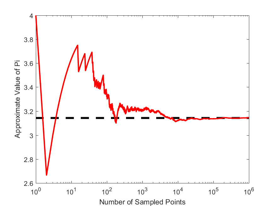
\[\pi \approx 4\frac{n_C}{n_{\rm total}}\]

Now, write a script that takes in the number of points to be simulated, and then calculates an approximate value for $\pi$ based on the Monte Carlo algorithm described above. Write a second function that plot the estimate of $\pi$ versus the number of points stimulated, like the following,

Solution

Here is an example MATLAB script that estimates $\pi$: estimatePi.m,

nsample = 1000000;
X = rand(nsample,2);
InsideCircle = ( X(:,1).^2 + X(:,2).^2 ) <= 1;
ApproximatePI = zeros( size(InsideCircle) );
sumInsideCircle = 0.0;
for isample = 1:nsample
    sumInsideCircle = sumInsideCircle + InsideCircle(isample) ;
    ApproximatePI(isample) = 4.0 * sumInsideCircle / isample ;
end
disp( [ 'Approximate value of PI for '...
        , num2str(nsample) ...
        , ' samples: ' ...
        , num2str(ApproximatePI(end)) ...
      ] ...
    );
figure(); hold on; box on;
line( [ 1 nsample ] ...
    , [ pi pi ] ...
    , 'linestyle' , '--' ...
    , 'linewidth' , 3 ...
    , 'color' , 'black' ...
    );
plot( ApproximatePI(2:end) ...
    , 'linewidth' , 2 ...
    , 'color' , 'red' ...
    );
xlabel( 'Number of Sampled Points' ) ;
ylabel( 'Approximate Value of Pi' ) ;
set( gca , 'XScale' , 'log' );
saveas( gcf, 'approximatePI.png' );

Here is an example Python code that estimates $\pi$,

import numpy.random as rnd
import numpy.linalg as nlg
import numpy as np
import matplotlib.pyplot as plt

def estimatePi(n=100000):
    x = np.zeros((n,4),dtype=np.dtype)
    counter = 0
    for i in range(n):
        x[i,0:2] = rnd.uniform(0.0,1.0,2)  # generate two uniform random numbers
        x[i,2] = nlg.norm(x[i,:], ord=2)
        if (x[i,2]<=1.0): counter += 1
        x[i,3] = 4.0*np.double(counter)/np.double(i+1)
    return x # the running approximate of pi is returned as a vector in the fourth column of x

def plotPi(n=10000):
    x = estimatePi(n)
    plt.semilogx( list(range(1,n+1)) \
                , x[:,3] \
                ) # plot with color red, as line
    plt.xlabel('Number of simulated points')
    plt.ylabel('Approximate value of Pi')
    #plt.axis([1, n , 0.1, 4.0]) # [xmin, xmax, ymin, ymax]
    plt.title('Estimating Pi by Monte Carlo simulation')
    plt.savefig('approximatePi_{}.png'.format(n))
    plt.show()

plotPi()