In probability theory, the central limit theorem (CLT) establishes that, when independent random variables are added together, their properly normalized sum tends toward a normal distribution (informally a “bell curve”) even if the original variables themselves are not normally distributed. To understand this theorem, suppose you generate 100 uniform random numbers and sum them to get a single number. Then you repeat this procedure 1000 times to get 1000 of these sums of 100 uniform random numbers. The CLT theorem implies that if you plot a histogram of the values of these 1000 sums, then the resulting distribution looks very much like the Gaussian bell-shaped function. The larger the number of these sums (for example, 100000 instead of 1000 sums), the more the resulting distribution will look like a Gaussian. Here we want to see this theorem in action.
Consider a random walker, who takes a random step of a uniformly-distributed random-size between $[0,1]$, in positive or negative directions on a single staright line. The random walker can repeat these steps for nstep times, starting from an arbitrary initial starting point.
Write a function with the interface doRandomWalk(nstep,startPosition), that takes the number of steps nstep for a random walk and the startPosition of the random walk on a straight line, and returns the location of the final step of the random walker.
Now, write another function with the interface simulateRandomWalk(nsim,nstep,startPosition) that simulates nsim number of random-walks, each of which contains nstep steps and starts at startPosition. Then, this function calls doRandomWalk() repeatedly for nsim times and finally returns a vector of size nsim containing final locations of all of the nsim simulated random-walks.
Now write a script that plots the output of simulateRandomWalk() for
The resulting plot should look like the following,
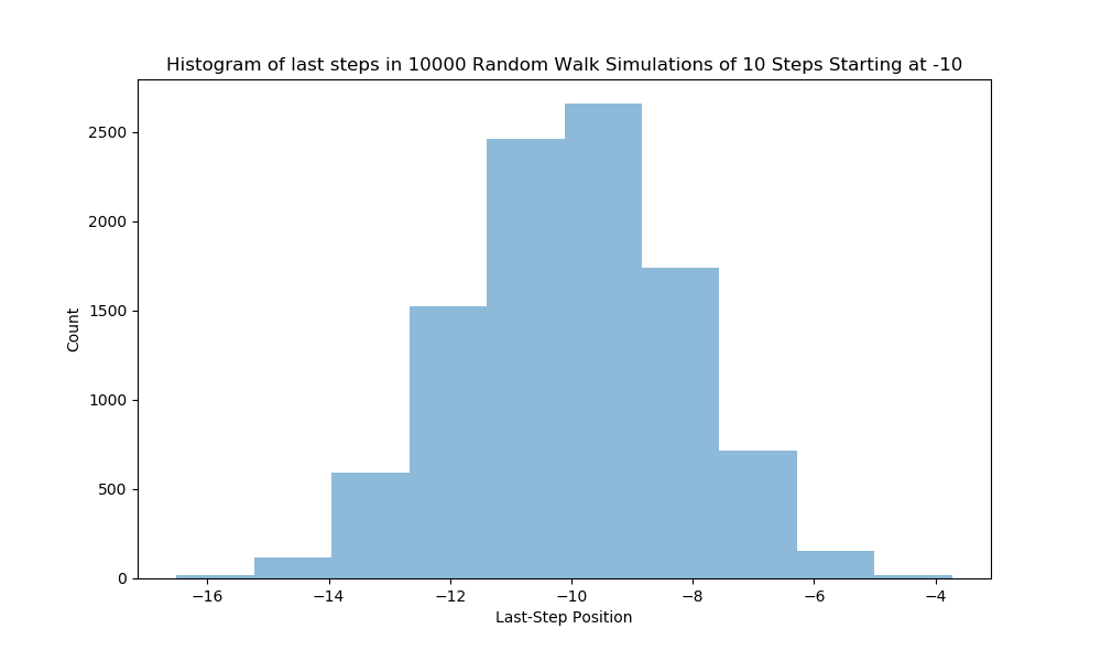
How do you interpret this result? How can uniformly-distributed random final steps end up having a Gaussian bell-shape distribution.