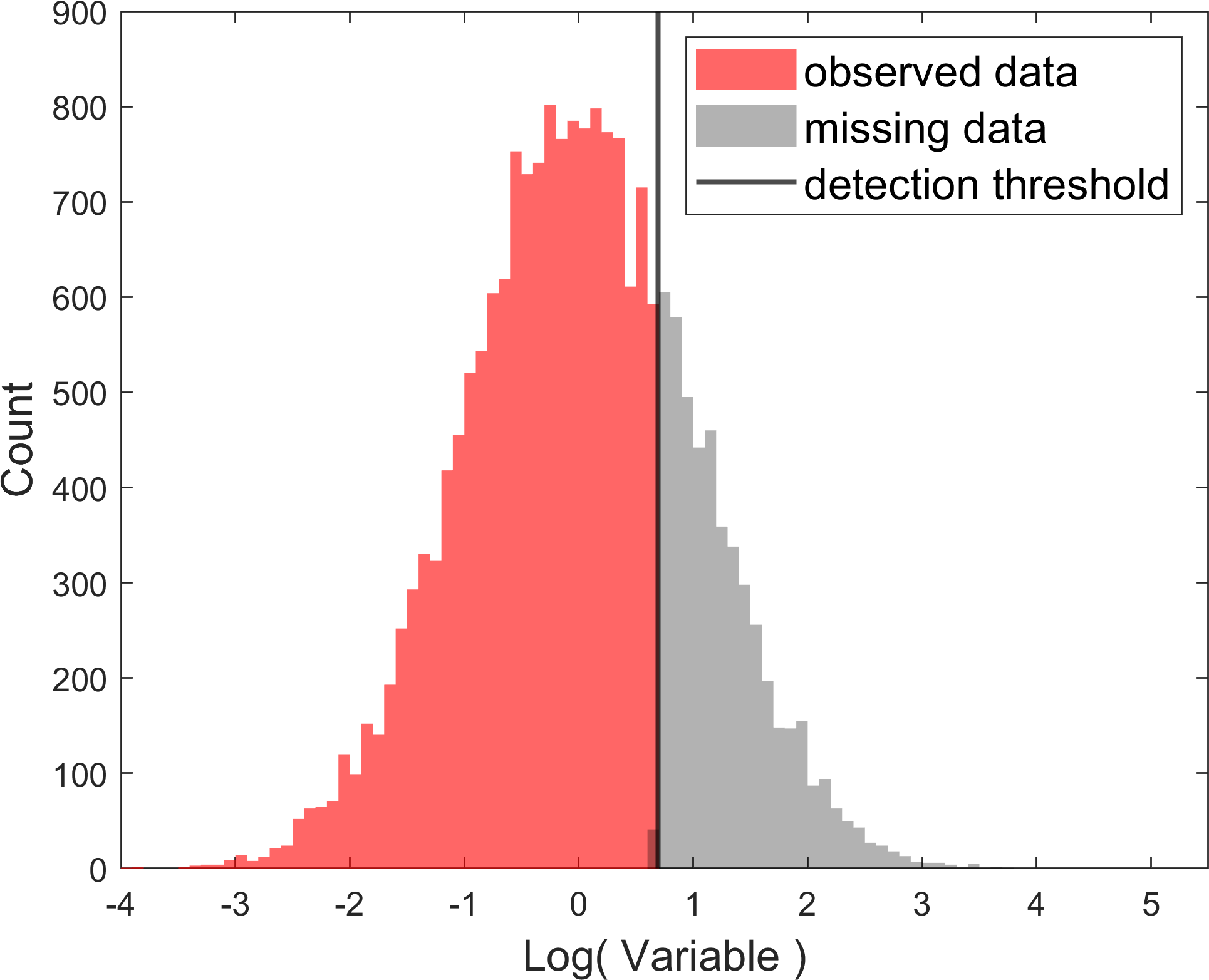
Supposed we have observed a dataset comprised of $15027$ events with one attribute variable in this file: data.csv. Plotting these points would yield a red-colored histogram like the following plot,

The pale black shaded area represents the missing points from our observational dataset. These are points that we could NOT observe (or detect) because of some instrumental bias and sample incompleteness as represented by the black line.
Now our goal is to form a hypothesis about this dataset, that is, a hypothesis about the distribution of the events in the above plot. To make a correct assessment, we will have to also carefully consider the effects of the detection threshold (the black line) in our inference.
To help you get started, we can first take the logarithm of this dataset to better understand the distribution of the attribute of the dataset and plot the transformed data,
Just by looking at the observed (red) distribution, we can form a relatively good hypothesis about the distribution of the data: If the detection threshold did not exist, the complete dataset (including the points in the black shaded area) would have likely very well resembled a lognormal distribution (or a normal distribution on the logarithmic axes).
However, this dataset is affected by the detection threshold and we need to also take a model of the detection threshold into account. The logarithmic transformation makes it crystal-clear to us that the detection threshold is likely best modeled by a vertical line.
Now, use the maximum likelihood method combined with the MCMC sampling technique in the language of your choice (e.g., Python/MATLAB) to perform a Markov Chain Monte Carlo simulation for this regression problem and find the underlying true parameters of the hypothesized lognormal distribution (or equivalently, the Gaussian distribution in logarithmic space) as well as the detection threshold value (the value of the vertical black line).
- To solve this problem, and any other scientific problem solving, We should always break it down to simpler tinier chunks that are manageable and also simplify the scientific hypothesis so that the possibility of accumulation of layers of error in the calculations diminishes. In this case, a simpler hypothesis than the censored Gaussian fit to this data is a simple Gaussian fit without any sample censorship. We will first solve this problem for this simple hypothesis of a uncensored Gaussian.
- First, write a function that takes an input observation and the parameters of a Gaussian distribution ($\mu, \sigma$) and returns the natural logarithm of the Gaussian probability density function (PDF),
\(\log\big( \pi( D_i | \mu, \sigma ) \big).\) - Use the simple generic definition of the likelihood function,
\(\begin{eqnarray*} \log\Big( \mathcal{L}\big( \mathcal{D}; \mathbf{\theta} = [\mu, \sigma] \big) \Big) &=& \log\Big( \prod_{i = 1}^{i = N} ~ \pi( D_i | \mu, \sigma ) \Big) \\ &=& \sum_{i = 1}^{i = N} ~ \log\Big(\pi( D_i | \mu, \sigma ) \Big) ~. \end{eqnarray*}\) - Maximize this liklelihood function to get the best-fit Gaussian parameters for the model. The best-fit model would yield a fit like the following to our data,
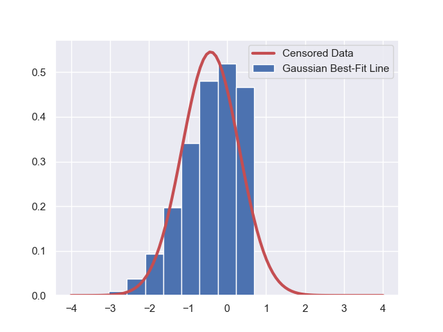
which despite being the best-fit, still looks quite awful. Why? Because our hypothesis is awful: This dataset is not pure Gaussian, it is censored. - We can now go on to the more sophisticated case that includes data censorship.
- First, write a function that takes an input observation and the parameters of a Gaussian distribution ($\mu, \sigma$) and returns the natural logarithm of the Gaussian probability density function (PDF),
Hint:
-
First read the data using Pandas library, then log-transform data to make it look like a Normal distribution.
-
Write a class or a series of functions that take the log-data as input and has two methods,
getLogProb(data,avg,std,cutoff)andgetLogLike(param). The former computes the log-probability of observing the input datasetdatagiven the parameters of the model (the Normal averageavg, the Normal standard deviationstd, and the vetical cutoff on the distributioncutoff). The latter method takes a set of parameters as a vector containing the average of the Normal distribution (avg), the natural-logarithm of the standard deviation of the Normal distributionlog(std), and the value of the hard-cutoff on the data. Given these three parameters,getLogLike(param)sums over the log-probabilities returned bygetLogProb(data,avg,std,cutoff)to compute the log-likelihood and returns it as the output. -
Think about this problem: If any of the observed data points has a value that is larger than a given hard-cutoff, could that set of parameters with that hard-cutoff be possible at all? In other words, if the maximum of your data is larger than the given input
cutoffvalue (which isparam[2]ingetLogLike()), then that set of input parameters togetLogLike()is impossible. Therefore, the log-likelihood corresponding to that set of parameters must be negative-infinity to indicate the impossibility of that set of parameters. However, given the computer’s limited float range, the log-likelihood must be set to the largest negative number (e.g.,-1.e300is good enough) and returned. Otherwise, if all data values are smaller than the input cutoff, then the log-likelihood value is computed by summing over all probabilities returned bygetLogProb(). -
In the latter case when you call
getLogProb(), keep in mind that you will have to normalize the log-Gaussian probabilities, that you would normally compute, by the incomplete area created by the hard cutoff on the distribution. This is the area to the left of the hard cutoff on the distribution and can be computed via the Gaussian Cumulative Distribution Function (CDF). You will have to subtract the natural logarithm of this area from the log-probabilities of all data. -
You can use the ParaMonte library in Python or in MATLAB to explore the resulting log-likelihood function. In such case, make sure you start your MCMC exploration by a good set of initial parameter values, such that the MCMC sampler can correctly explore the parameter-space without getting lost. This means making sure that you set the initial starting cutoff value to something larger than the maximum value of your data, for example,
cutoff_init = 2 * np.max(logdata). Here is the full syntax on how to call theParaDRAM()sampler of theparamontelibrary,
import paramonte as pm
pm.version.interface.dump() # get the version of ParaMonte we are working with
pmpd = pm.ParaDRAM() # create a ParaDRAM sampler object
pmpd.spec.chainSize = 20000 # change the number of sampled points from default 100,000 to 30,000
pmpd.spec.variableNameList = ["Average","LogStandardDeviation","Cutoff"]
pmpd.spec.startPointVec = [0,0,normal.maxdata] # ensure the initial starting point of the search for cutoff is good.
pmpd.spec.targetAcceptanceRate = [0.1,0.3] # ensure the MCMC sampling efficiency does not become too large or too small.

# call MCMC sampler

pmpd.runSampler( ndim = 3
               , getLogFunc = normal.getLogLike
               )
ParaDRAM - NOTE: Running the ParaDRAM sampler in serial mode...
ParaDRAM - NOTE: To run the ParaDRAM sampler in parallel mode visit: cdslab.org/pm
ParaDRAM - NOTE: If you are using Jupyter notebook, check the Jupyter's terminal window
ParaDRAM - NOTE: for realtime simulation progress and report.


ParaDRAM - NOTE: To read the generated output files sample or chain files, try the following:
ParaDRAM - NOTE:
ParaDRAM - NOTE:     pmpd.readSample()      # to read the final i.i.d. sample from the output sample file.
ParaDRAM - NOTE:     pmpd.readChain()       # to read the uniquely-accepted points from the output chain file.
ParaDRAM - NOTE:     pmpd.readMarkovChain() # to read the Markov Chain. NOT recommended for extremely-large chains.
ParaDRAM - NOTE:
ParaDRAM - NOTE: Replace 'pmpd' with the name you are using for your ParaDRAM object.
ParaDRAM - NOTE: For more information and examples on the usage, visit:
ParaDRAM - NOTE:
ParaDRAM - NOTE:     https://www.cdslab.org/paramonte/
where normal.maxdata represents the maximum of the data, and normal.getLogLike(param) returns the log-likelihood value given the input param which is the average and log-standard-deviation of the Normal distribution and the cutoff, corresponding to param[0], param[1], param[2].
Here is the resulting maximum-likelihood parameters inferred from the paramonte-ParaDRAM MCMC sampler as is done below in Python:
sample = pmpd.readSample(renabled = True)[0]
sample.df.mean()
SampleLogFunc -38794.057165
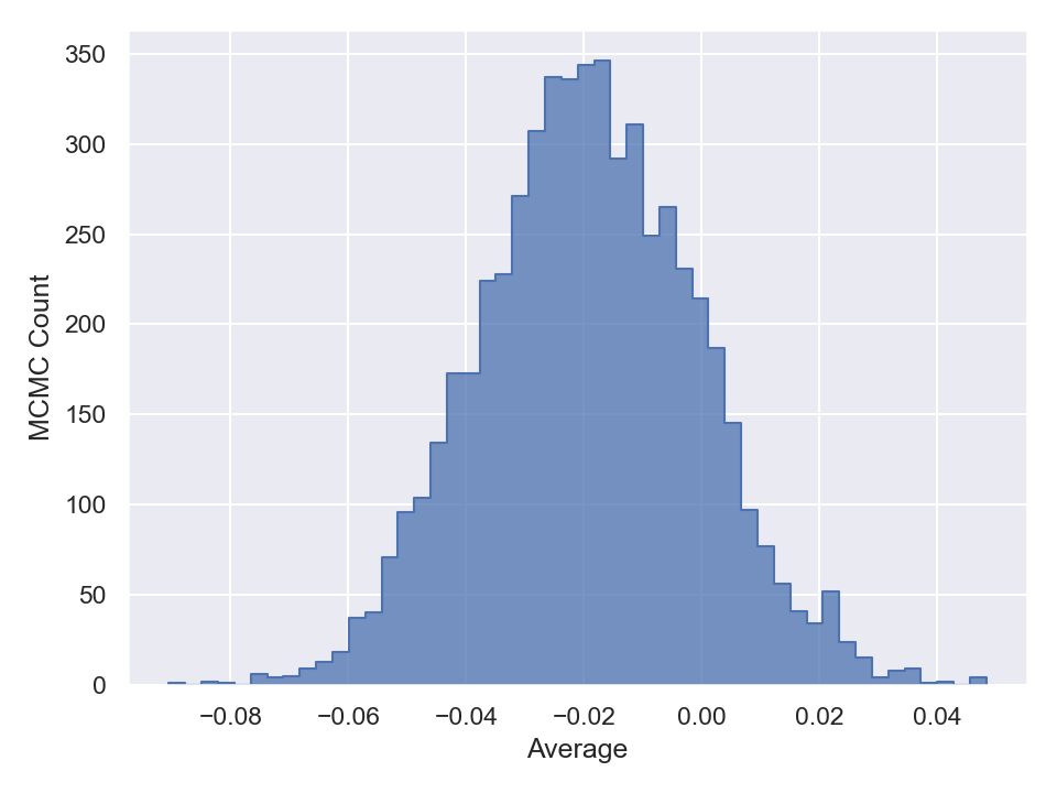
Average -0.018469
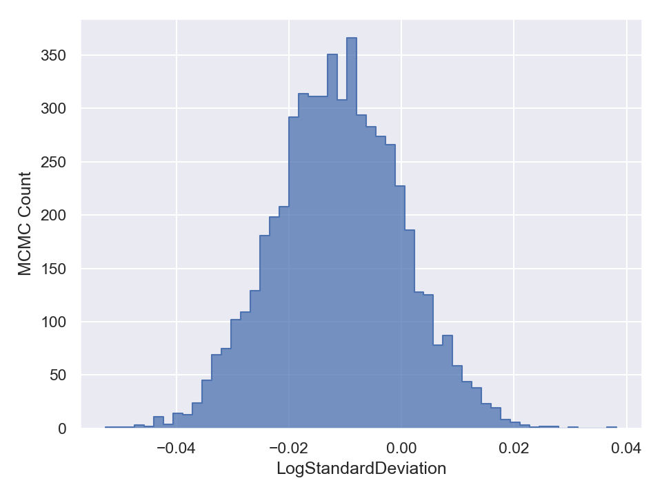
LogStandardDeviation -0.011038
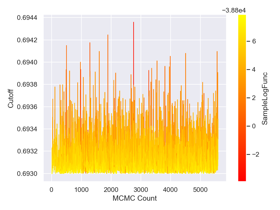
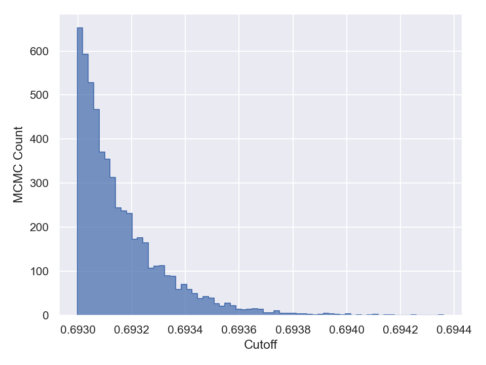
Cutoff 0.693154
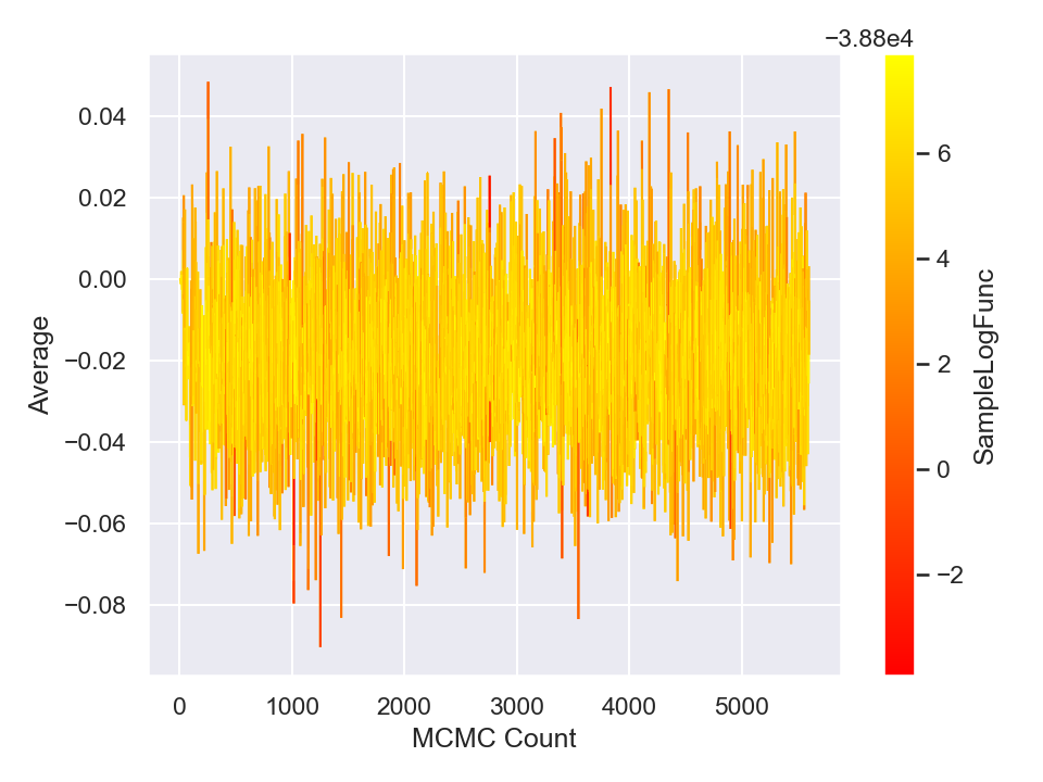
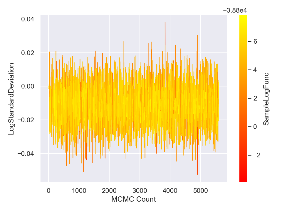
Once you are done with sampling, you can draw and save the parameter traceplots and histograms like the following (in Python),
# read the resulting sample

sample = pmpd.readSample(renabled = True)[0]

# plot traceplots of the sampled parameters

for colname in sample.df.columns:
    sample.plot.line.ycolumns = colname
    sample.plot.line.outputFile = "traceplot_" + colname
    sample.plot.line()
    sample.plot.line.currentFig.axes.set_xlabel("MCMC Count")
    sample.plot.line.currentFig.axes.set_ylabel(colname)

# plot the histograms of the sampled parameters

for colname in sample.df.columns:
    sample.plot.histplot.columns = colname
    sample.plot.histplot.outputFile = "histogram_" + colname
    sample.plot.histplot()
    sample.plot.histplot.currentFig.axes.set_xlabel(colname)
    sample.plot.histplot.currentFig.axes.set_ylabel("MCMC Count")
This will generate and save to external files, the following plots,
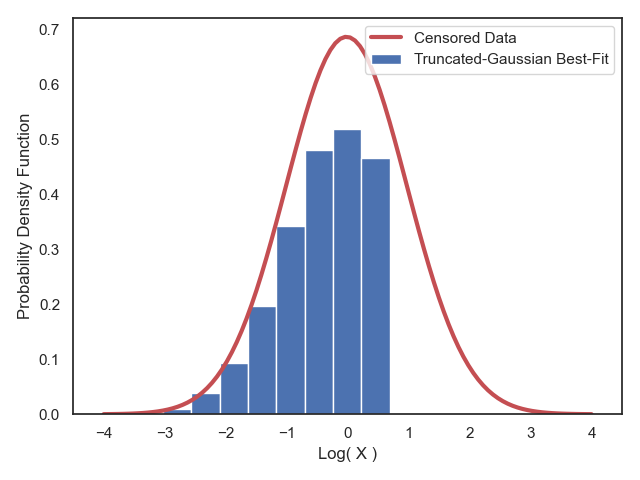
Here is a plot of the resulting best-fit truncated Gaussian to the censored data: