Computing the cross-correlation of two data attributes

Problem

Consider this dataset of carbon emissions history per country.

Make a visualization of the global carbon emission data in the CSV file in the above by summing over the contributions of all countries per year to obtain an illustration like the following,
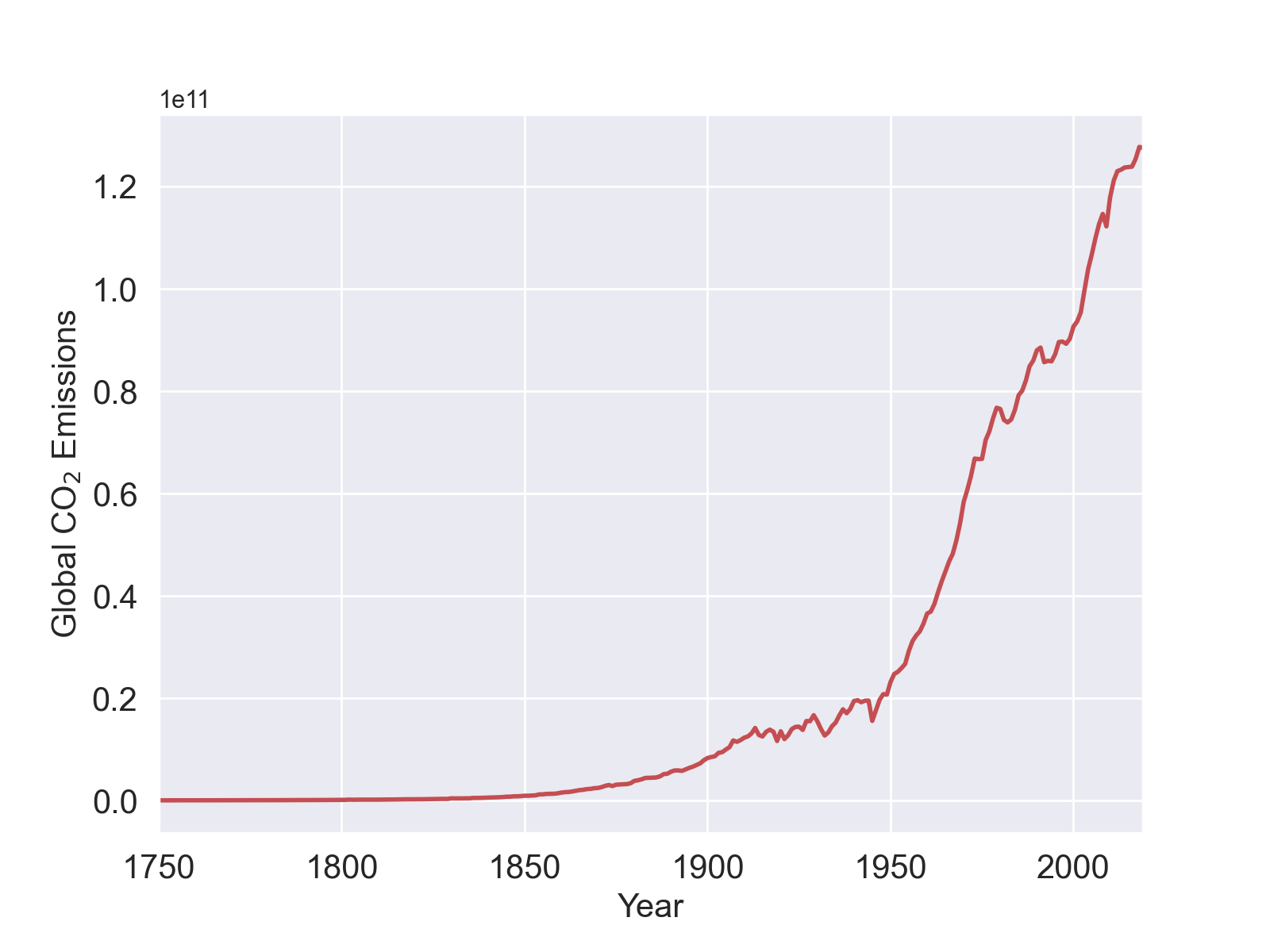
Now consider the contribution of individual countries in this zero-filled CSV dataset and make a stacked plot of the countries over the years, like the following,

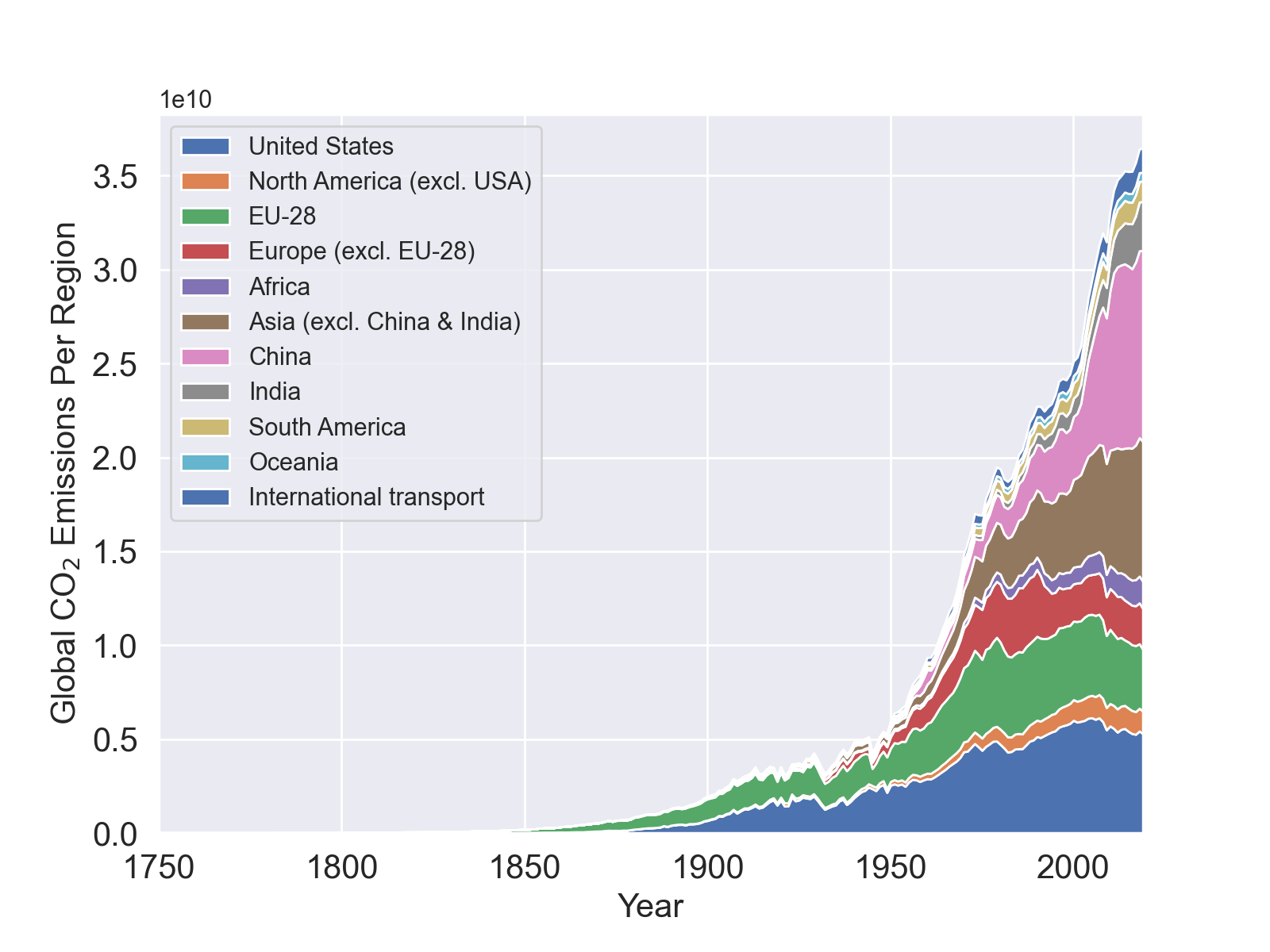
To do so, you will have to extract the data for the following regions from the CSV file and matplotlib stackplot in Python or some other similar package or function in your language of choice.
Recall the globalLandTempHist.txt dataset that consists of the global land temperature of Earth over the past 300 years. Parse the contents of this file to generate the average annual temperature anomaly data. Then, extract the subset of CSV data from Step 2 in the above corresponding to the regional keyword "World" in the Entity column of data. Then, match the temperature anomaly data with the global CO2 emission data to generate a unified dataset. Then, write a function that computes the cross-correlation between the temperature anomaly and the global CO2 emissions. Use the definition of the correlation matrix that we have seen before to compute the cross-correlation.
Now, use an external library in the language of your choice to compute the autocorrelation using Fast-Fourier Transform (FFT). Within Python, you can use correlate in SciPy package from scipy.signal import correlate to compute the autocorrelation. To do so, you will have to first normalize the input data (the anomaly data) to its mean. Then you pass the data in syntax like the following,
```
import numpy as np
from scipy.signal import correlate

anomalies = anomalies - np.mean(anomalies)
emissions = emissions - np.mean(emissions)

nlag = len(anomalies) - 1
acf = np.zeros(nlag)

acf = correlate ( anomalies
                , emissions
                , mode = "full"
                )[nlag:2*nlag]
acf = acf / acf[0]
```
Make a plot of this autocorrelation function (acf) and compare with what you have obtained from the slow version you have implemented.

Computing the cross-correlation of two data attributes

Problem

Amir Shahmoradi

Comments